Week 3 - Solving second order ODEs
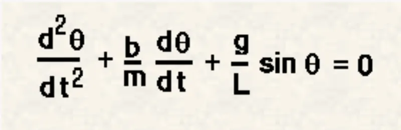
Aim: To write a program that solves the following ODE which represents the equation of motion of a simple pendulum with damping.
ODE:
CODE:
clear all
close all
clc

%Inputs for pendulum
b=0.09;                         %Damping Coefficient of pendulum.
m=0.1;                          %Mass of bob.
g=9.81;                         %Accelaration due to gravity.
L=1;                            %Length of string which is massless.

%Intial conditions
theta_0=[0 5]                   %Since there are two first ODE, so the intial conditions for the displacement is '0' and initial condition for velocity is '5'.

t_span=linspace(0,10,500);      %Time array starting from '0' to '10'.

[t,results] = ode45(@(t,theta) ode_func(t,theta,b,g,L,m),t_span, theta_0);     %ode45 is an inbuilt function in matlab which helps to determine the values of the ODE.
                                                                               %where the main inputs are 't' and 'theta'. Syntax 'ode45(odefun,tspan,y0)'.
                                                                               %Since we are solving two ODEs we get 2 column vectors, which will be stored in 'results'.

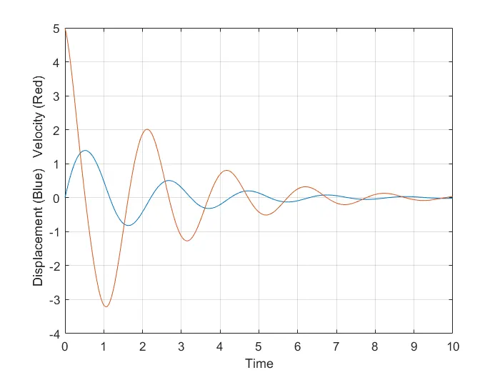
plot(t,results(:,1))            %Displacement plot of the pendulum.
hold on
plot(t,results(:,2))            %Velocity plot of the pendulum.

xlabel('Time')                  %X-axis.
ylabel('Displacement (Blue)   Velocity (Red)') %Y-axis.
grid on
FUNCTION CODE OF THE ABOVE CODE:
function [dtheta_dt] = ode_func(t,theta,b,g,l,m)   %Function definition.

   theta1 = theta(1);           %Since theta is our solution array, we clubed both 'theta1' and 'theta2' into theta. So 'theta of 1' is 'theta1'.
   theta2 = theta(2);           % and 'theta of 2' is 'theta2'.

   dtheta1_dt = theta2;                            %Our first 1st degree ODE.
   dtheta2_dt = -(b/m)*theta2 - (g/l)*sin(theta1); %Our second 1st degree ODE.

   dtheta_dt = [dtheta1_dt;dtheta2_dt];   % Combined the above the results into an array
                                            by sepearting it into columns.
end
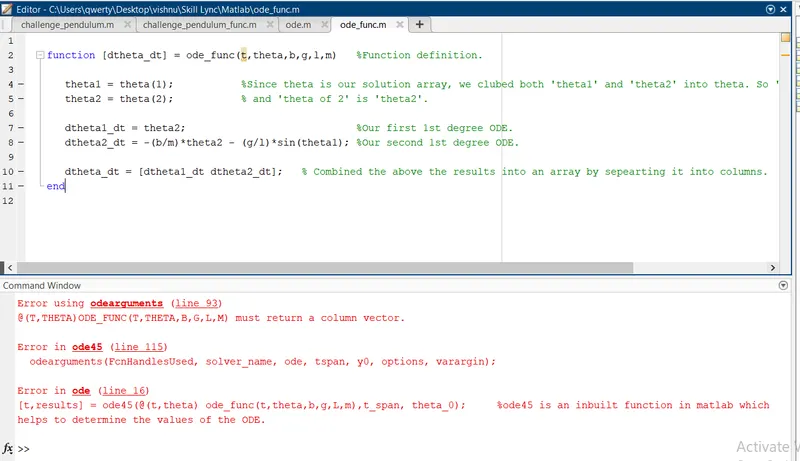
ERRORS FACED WHILE CODING:
1) Error using odearguments (line93).
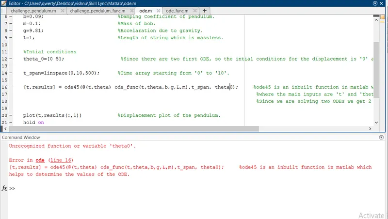
2) Unrecognized function or variable 'theta0'.
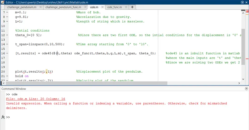
3) Invalid expression. When calling a function or indexing a variable (line 20).
STEPS TAKEN TO OVERCOME THESE ERRORS:
1) ';' was added between 'dtheta1_dt' and 'dtheta2_dt' since it was in column matrix.
2) 'theta0' was corrected as 'theta_0'.
3) ';' was replaced by ':'.
SCREENSHOTS SHOWING THE ERRORS:
1)
2)
3)
RESULT:
Succesfully coded the program that solves the above ODE which represents the equation of motion of a simple pendulum with damping.
PLOT:
INFERENCE:
Its clearly evident from the graph that when velocity becomes zero the displacement achieves nearly peak.
PENDULUM PROBELM
AIM: Write a program in Matlab that will simulate the pendulum motion ,use L=1 metre,m=1 kg,b=0.05,g=9.81 m/s2 and
simulate the motion between 0-20 sec, for angular displacement=0,angular velocity=3 rad/sec at time t=0.
ODE: ODE is same the above.
CODE:
clear all
close all
clc

%Intializing the values of pendulum
L = 1.5;                       %Length of pendulum which is massless.
g = 9.81;                      %Accelaration due to gravity.
b = 0.05;                      %Damping Coefficient.
m = 1;                         %Mass of bob.

ct = 1;                        %Counter set count the frames while making the movie.

theta_0 = [0;3];               %Since there are two first ODE, so the intial conditions for the displacement is '0' and initial condition for velocity is '3'.
t_span = linspace(0,20,500);   %Time array starting from '0' to '20'

[t,result] = ode45(@(t,theta)challenge_pendulum_func(t,theta,L,g,b,m),t_span,theta_0);  %ode45 is an inbuilt function in matlab which helps to determine the values of the ODE.
                                                                                        %where the main inputs are 't' and 'theta'. Syntax 'ode45(odefun,tspan,y0)'.
                                                                                        %Since we are solving two ODEs we get 2 column vectors, which will be stored in 'results'.


pendulum= result(:,1);          %Since the 'result' is an array we use another variable 'pendulum' which stores the values of 'result', so that we can use the length of 'pendulum' in next step.
for i=1:length(pendulum)        %Used the 'length' operator to find the length of pendulum.
    pendulum1 = pendulum(i);    %Assigned each value of 'pendulum(i)' to 'pendulum1'

    x0 = 0;                     %Starting X Coordinate of pendulum string.
    y0 = 0;                     %Starting Y Coordinate of pendulum string.
    x1 = L*sin(pendulum1);      %Ending X Coordinate of pendulum string.
    y1 = -L*cos(pendulum1);     %Ending Y Coordinate of pendulum string.


    plot([-1 1],[0 0],'linewidth',4,'color','g')       %Rigid rod which helps in support of pendulum to oscilate.
    axis([-2 2 -2 2])           %Representing the axis in the plot.
    hold on
    grid on
    plot([x0 x1],[y0 y1],'linewidth',2,'color','b')    % Plotted the string of the Pendulum.
    plot(x0,y0,'H','markersize',10,'MarkerEdgeColor','g','MarkerFaceColor','r'); %plotted the connection between pendulum string and rigid rod.
    plot(x1,y1,'O','markersize',30,'MarkerEdgeColor','g','MarkerFaceColor','r'); %Plotted the Bob of pendulum.

    pause(0.03)                % A pause of '0.03' seconds. It will be executed in every loop.

    hold off
    M(ct) = getframe(gcf);     %'getframe' command captures the entire interior of the current figure window.
    ct = ct+1;
end
movie(M)
videofile = VideoWriter('Challenge_Pendulum','Uncompressed AVI');
open(videofile)
writeVideo(videofile,M)
close(videofile)
FUNCTION CODE OF THE CODE:
function [dtheta_dt] = challenge_pendulum_func(t,theta,L,g,b,m)  %Function definition.

         theta1 = theta(1);                    %Since theta is our solution array, we clubed both 'theta1' and 'theta2' into theta. So 'theta of 1' is 'theta1'.
         theta2 = theta(2);                    % and 'theta of 2' is 'theta2'.

         dtheta1_dt = theta2;                  %Our first 1st degree ODE.
         dtheta2_dt = (-b/m)*theta2 - (g/L)*sin(theta1); %Our second 1st degree ODE

         dtheta_dt = [dtheta1_dt;dtheta2_dt];  %Combined the above the results into an array by sepearting it into columns.
end
ERRORS FACED WHILE CODING:
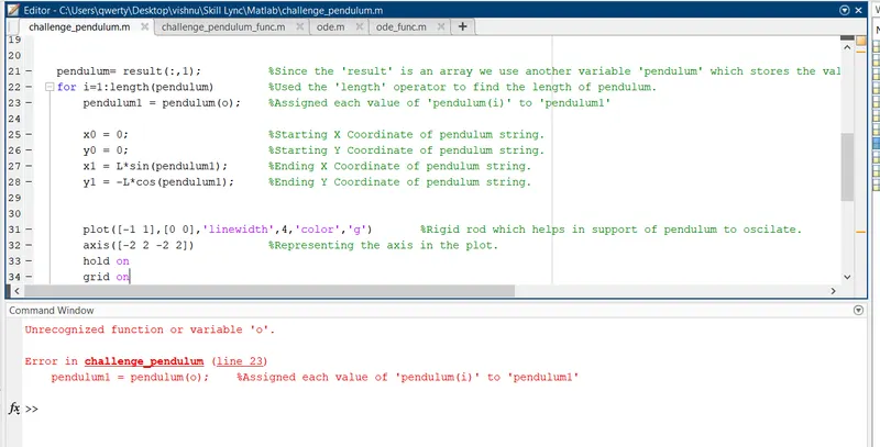
1) Unrecognized function or variable 'o'.
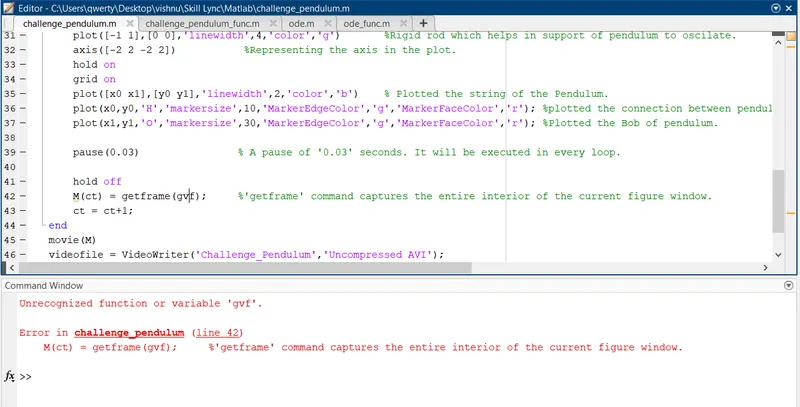
2) Unrecognized function or variable 'gvf'.
STEPS TAKEN TO OVERCOME THESE ERROS:
1) Replaced 'i' instead of 'o'.
2) Replaced 'gcf' instead of 'gvf'.
SCREENSHOTS SHOWING THE ERRORS:
1)
2)
LINK FOR THE ANIMATION:
RESULT:
Successfully coded the program in Matlab which will simulate the motion of simple pendulum.
INFERENCE:
Its is clear that when displacement is maximum velocity is zero and vice-versa.