Solving second order ODEs

Introduction:

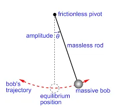
A pendulum is a weight suspended from a pivot so that it can swing freely. When a pendulum is displaced sideways from its resting, equilibrium position, it is subject to a restoring force due to gravity that will accelerate it back toward the equilibrium position.

Aim:

• To create a program for the second order differential equations which represents the motion of a simple pendulum.
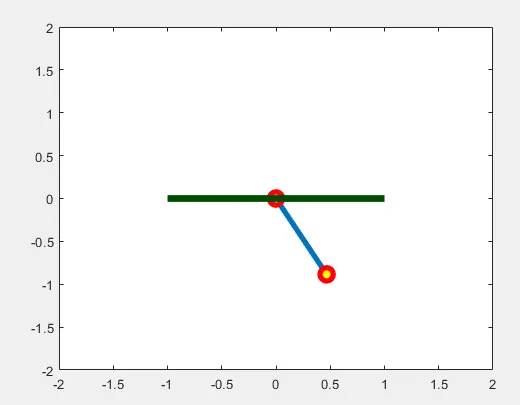
• To create a animation movie for the same.

Objective:

To create a Matlab program for ODE.

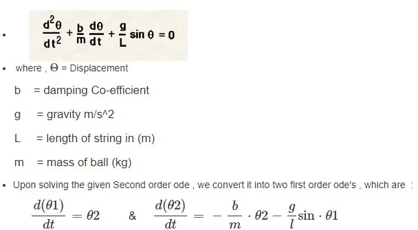
This ODE represents the simple motion of a pendulum.

Function Code:

% ODE Function
function dtheta_dt=ode_funs(t,theta,b,g,l,m);
theta1=theta(1);
theta2=theta(2);
dtheta1_dt=theta2;
dtheta2_dt=-(b/m)*theta2-(g/l)*sin(theta1);
dtheta_dt=[dtheta1_dt;dtheta2_dt];
end

• In this, the second order differential equation is simplified into first order differential equation.
• then theta1 & theta2 are differentiated and dtheta_dt value is obtained in column matrix.

Main Program:

clear all
close all
clc

% fixed parameters
b=0.05;      %Damping coefficient
g=9.81;      %Acceleration due to gravity(mts/s^2)
m=1;         %Mass(Kg)
l=1;         %length(mts.)

% Initial Conditions
theta_0=[0;3];

% Time points
tspan=linspace(0,20,200);

% Solving the ODE
[t,results]=ode45(@(t,theta)ode_fun(t,theta,b,g,l,m),tspan,theta_0);

% Plotting

%1st plot
figure(1)
plot(t,results(:,1))
hold on
plot(t,results(:,2))
xlabel('time')
ylabel('Velocity(RED) & Displacement(BLUE)')

%2nd plot
ct=1;
for i=1:length(results(:,1))
    x0=0;
    y0=0;
    x1=1*sin(results(i,1)+pi);
    y1=1*cos(results(i,1)+pi);
    figure(2)
plot([x0 x1],[y0 y1],'-o','MarkerSize',10,'MarkerFaceColor','y','MarkerEdgeColor','r','linewidth',4)
axis([-2 2 -2 2])
hold on
plot([-1  1],[0 0],'linewidth',5,'color','[0 0.3 0]')
M(ct)=getframe(gcf);
hold off
ct=ct+1;
end
% Movie & VideoFile
movie(M)
v_f=VideoWriter('Pendulum_challenge.avi','Uncompressed AVI')
open(v_f)
writeVideo(v_f,M)
close(v_f)

• In this program, the fixed parameters are length, mass, damping coeff, acce due to gravity.
• Time and angle are given as the initial conditions.
• In the tspan command, 200 values are taken in between 0-20.
• using the ode45 command ODE is introduced.
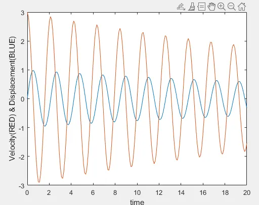
• Using plot command velocity & displacement v/s time graph is plotted.
• Using the for loop the mass at various points and various times are marked in the graph
• Using the movie command the plot is saved as an uncompressed avi file.

Plot:

Animation: