Parsing NASA thermodynamic data

Aim:

• To extract all the coefficients of the species mentioned in the data file and calculate their parameters like enthalpy, entropy, and specific heat.
• To plot the variation of these parameters for the specified local temperature range
• To determine the molecular masses of the individual species mentioned in the data file.

Procedure:

• Initially open the given thermodynamic data file and read the data in the file and store the data to the variable F.
• Then read the header file of thermodynamic data and calculate the global low,mid and high temperature from the second line of header file.
• By using fgetl(), strsplit() and str2num() command find out the global low,mid and high temperatures in the second line.
• Then calculate the 14 coefficients for all the species in the given thermodynamic data file.
• In data file each species has three lines in which 14 coefficients are there.
• 6 By using the for loop, calculate the 14 coefficients for all the species.
• By using strfind() command, find out the number of exponential in first line, by which we can find out the number of coefficient in first line.
• Once you find out, then convert the coefficient from string form to number form by using str2num() command.
• By doing the above steps for line two and three, we can calculate the 14 coefficients for all the species.
• Once you find out the coefficients for a species, then calculate the entropy,enthalpy and specific heat.
• First 7 coefficients are high temperature coefficients and calculate cp,H and s.
• Assuming universal gas constant R=8.314 J/mol-k and assuming temperature range from 100 to 5000 take 100 values by linspace() command.
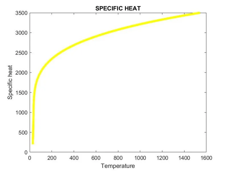
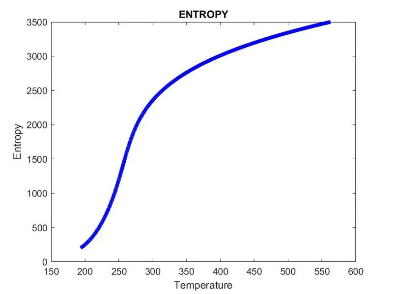
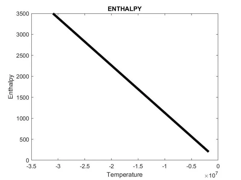
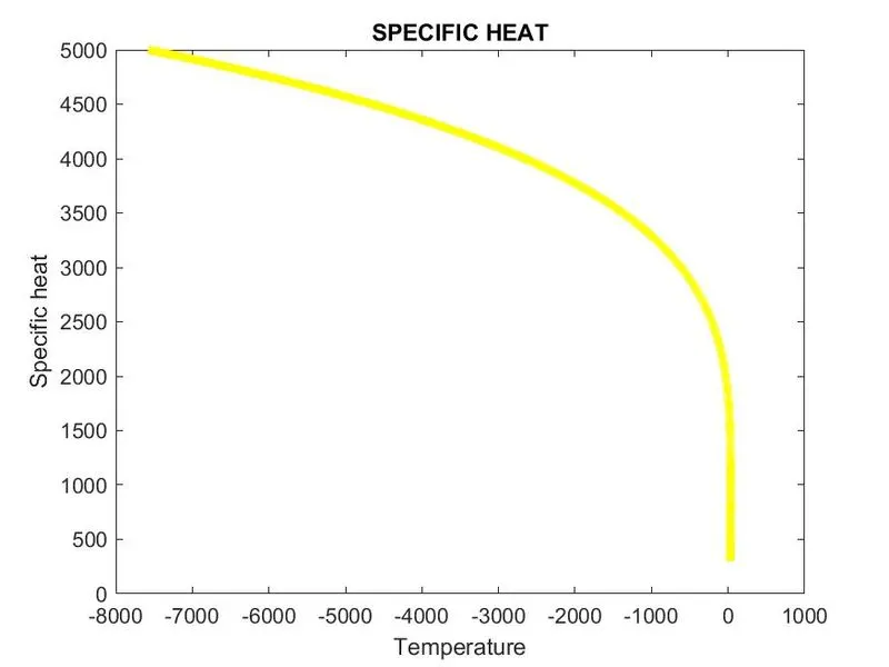
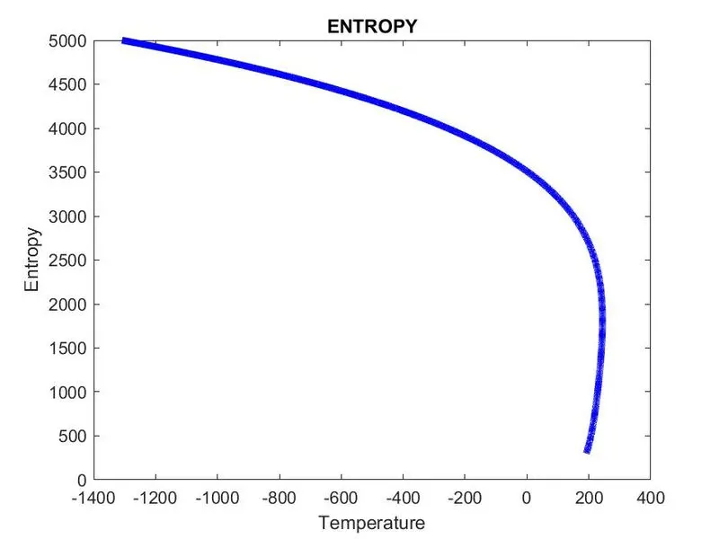
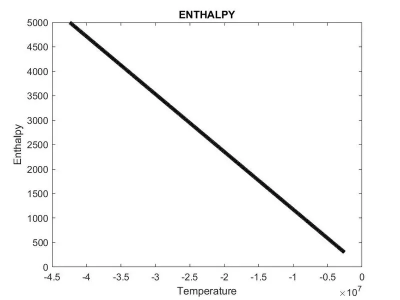
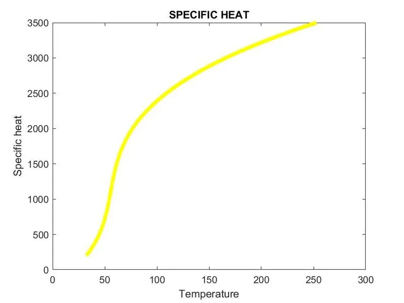
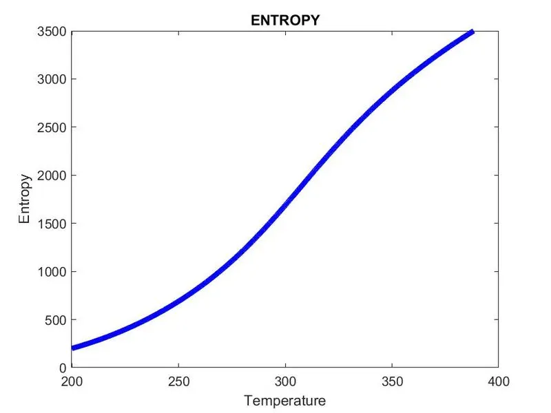
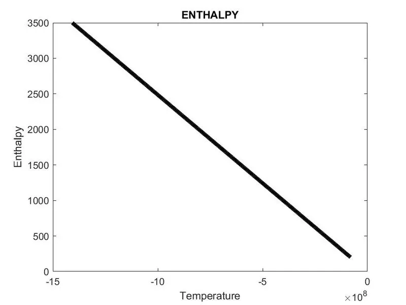
• Once you calculate the entropy,enthalpy and specific heat for all the species, plot the graph between: Temperature vs Entropy, Temperature vs Enthalpy and Temperature vs Specific heat.
• Store all the three plots for all the species in the file. The stored file is shown in the above picture.
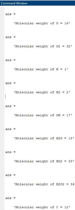
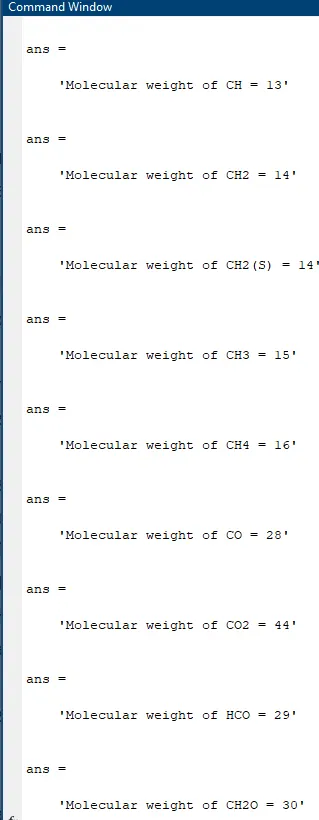
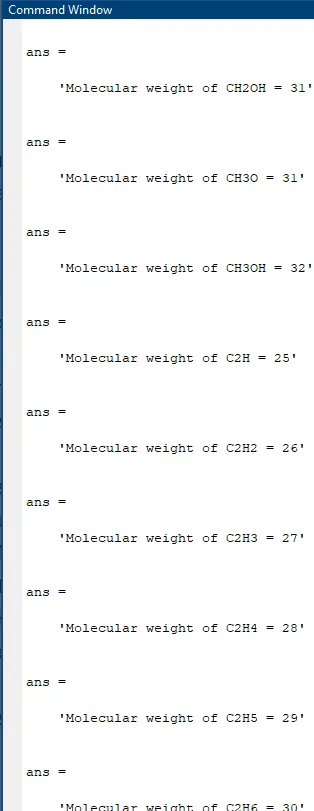
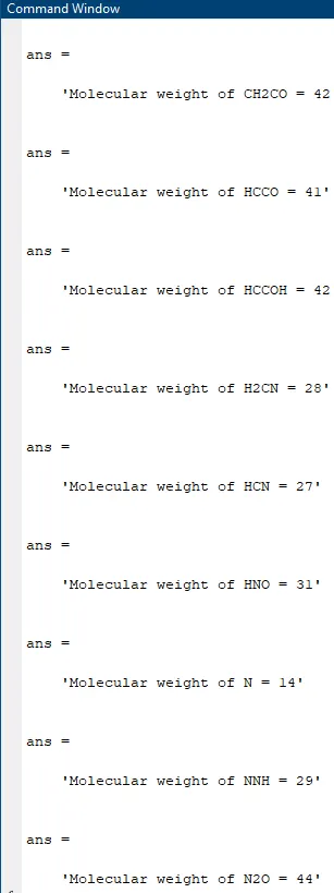
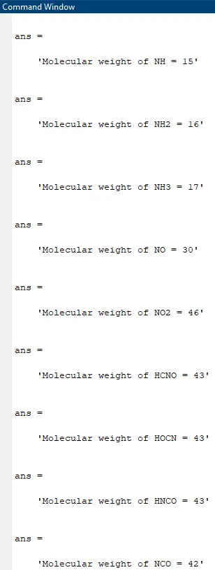
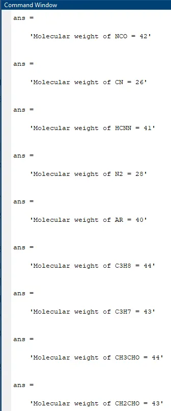
• Finally calculating the molecular weight for all the species and displayed in the command window.
• The method for calculating molecular weight is shown in the function program.

Code:

1. Primary Parsing Code:

clear all
close all
clc

f1=fopen('THERMO.dat','r');
tline=fgetl(f1);

%Universal gas constant(J/K mol)
R=8.314;

%Loop to run the first 4 lines of the data file
for i=1:4
    fgetl(f1);
end

%Loop to obtain data and get the plots for each species
for i=1:53
    
     %Obtaining the name of the species and converting to a string value
    %for convenience
    tline1=fgetl(f1); 
   
a=strsplit(tline1,' ');
species_cell=a(1);
species=char(species_cell);

%Finding the local values of temperature for each species
str1=strfind(tline1,'.');
low_temp_range=str2double(tline1(str1(1)-4:str1(1)+3));
high_temp_range=str2double(tline1(str1(2)-4:str1(2)+3));
mid_temp_range=str2double(tline1(str1(3)-4:str1(3)+3));

 %Obtaining the coefficients from the subsequent three lines    
tline2=fgetl(f1);
str=strfind(tline2,'E');
str = strfind(tline2, 'E');
    a1 = str2num(tline2(1:str(1)+3));
    a2 = str2num(tline2(str(1)+4:str(2)+3));
    a3 = str2num(tline2(str(2)+4:str(3)+3));
    a4 = str2num(tline2(str(3)+4:str(4)+3));
    a5 = str2num(tline2(str(4)+4:str(5)+3));
    
    tline3 = fgetl(f1);
    a6 = str2num(tline3(1:str(1)+3));
    a7 = str2num(tline3(str(1)+4:str(2)+3));
    a8 = str2num(tline3(str(2)+4:str(3)+3));
    a9 = str2num(tline3(str(3)+4:str(4)+3));
    a10 = str2num(tline3(str(4)+4:str(5)+3));
    
    tline4 = fgetl(f1);
    a11 = str2num(tline4(1:str(1)+3));
    a12 = str2num(tline4(str(1)+4:str(2)+3));
    a13 = str2num(tline4(str(2)+4:str(3)+3));
    a14 = str2num(tline4(str(3)+4:str(4)+3));
    
%a1-a7 are low temperature coefficients, a8-a14 are high temperature
    %coefficients
    
     %Calculating molecular weight of each species
     molecular_wt= molecular_weight(species);
    sprintf('Molecular weight of %s = %d',species, molecular_wt)
    
%Defining T
T=low_temp_range:high_temp_range;

 %Obtaining the values for Cp, enthalpy and entropy using the coefficients 
if (T>mid_temp_range)
    
  Cp = R*(a1 + (a2*T) + (a3*(T.^2)) + (a4*(T.^3)) + (a5*(T.^4)));
        %Enthaply
        H = R*(a1 + (a2*T/2) + (a3*(T.^2)/3) + (a4*(T.^3)/4) + (a5*(T.^4)/5) + (a6*(T)));
        %Entropy
        S = R*((a1*log(T)) + (a2*T) + (a3*(T.^2)/2) + (a4*(T.^3)/3) + (a5*(T.^4)/4) + a7);
        
else
    %specific heat
        Cp = R*(a8 + (a9*T) + (a10*(T.^2)) + (a11*(T.^3)) + (a12*(T.^4)));
        %Enthaply
        H = R*(a8 + (a9*T/2) + (a10*(T.^2)/3) + (a11*(T.^3)/4) + (a12*(T.^4)/5) + (a13*(T)));
        %Entropy
        S = R*((a8*log(T)) + (a9*T) + (a10*(T.^2)/2) + (a11*(T.^3)/3) + (a12*(T.^4)/4) + a14);
       
        
  

end

%Creating the folder for the species
t=sprintf('%s',species);

mkdir(t);

 %Going in to the folder of the species to save the plots
cd(t)

%PLOTTING

% Entropy  v/s Temperature 
figure(1)
plot(S,T,'linewidth',4,'color','b')
title('ENTROPY')
xlabel('Temperature')
ylabel('Entropy')
saveas(gcf,'H.jpg')

%Enthalpy v/s Temperature 
figure(2)
plot(H,T,'linewidth',4,'color','k')
title('ENTHALPY')
xlabel('Temperature')
ylabel('Enthalpy')
saveas(gcf,'S.jpg')

%Specific heat v/s Temperature 
figure(3)
plot(Cp,T,'linewidth',4,'color','y')
title('SPECIFIC HEAT')
xlabel('Temperature')
ylabel('Specific heat')
saveas(gcf,'Cp.jpg')


%Going back to the previous directory
cd .. ;

         

end

2. Code to calculate the molecular masses of individual species:

function [m_wt] = molecular_weight(species)

%Defining the elements
elements=['H','C','N','O','R']; 

%Atomic weights of each element
Atomic_Weight = [1 12 14 16 40]; 
m_wt=0; 

%Looping for each element inside each species and finding the atomic weight
for i=1:length(species) 
    for j=1:length(elements) 
        if strcmp(species(i),elements(j)) 
           m_wt= m_wt + Atomic_Weight(j); 
            p=j; 
        end
    end
    %loop to multiply the coefficients of the elements if greater than 1.
    n=str2double(species(i)); 
    if n>1 
        m_wt = m_wt + (Atomic_Weight(p))*(n-1); 
    end
end

end

Images:

1. Location of species folder in desktop:

2. Molecular masses displayed in the command window:

Plots:

For O2:

For N2:

For Co2:

Conclusion:

• The characteristic curves for all the species are obtained.
• N2 and O2 follow the same general pattern with the only difference being that O2 gives out energy (positive enthalpy) and N2 takes in energy (negative enthalpy). Their relation to Temperature is as expected as they follow a parabolic path for Cp and S and a linear plot for H since Cp and S are inversely proportional to temperature and H is directly proportional to it.