Week 3 - Solving second order ODEs

Objective: Writing a program in MATLAB that will simulate the pendulum motion for given span of time and given angular acceleration and velocity, with these results of angular velocity of pendulum over the time, we need to animate the pendulum motion.

Simple Pendulum:

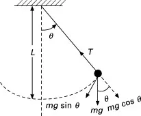
Using the mass-spring-damper system method, a simple pendulum motion can be described using the equation of motion as:

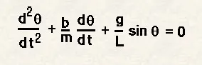
In the above equation,

• b = damping coefficient.
• g = gravity in m/s^2.
• L = length of the pendulum in the meter.
• m = mass of the ball in kg.

Input as per the problem statements:

• b = 0.05; # Damping Coefficient
• g = 9.81; # Gravitational Force in m/s^2
• l = 1; # Length of pendulum in m
• m = 0.1; # Mass in Kg
• Start angular displacement in rad.
• Start angular velocity in rad/sec^2
• Time of oscillation - 0 to 20 secs

Python Code:

"""

Challenge - 3 - solving 2nd order ODE to describe the transient behavior of simple pendulum

"""

import numpy as np

from scipy.integrate import odeint

import matplotlib.pyplot as plt

import math

from PIL import Image # to open each image in the current folder/ directory.

import glob # for animating set of image files

import natsort # To sort the whole image array in ascending order

# function that returns dz/dt

def model(theta,t,b,g,l,m):

theta1 = theta[0]

theta2 = theta[1]

dtheta1_dt = theta2

dtheta2_dt = -((b/m)*theta2) - ((g/l)*math.sin(theta1))

dtheta_dt = [dtheta1_dt, dtheta2_dt]

return dtheta_dt # returning the calculated values to function

# Inputs as per problem statement

b = 0.05 # Damping coefficient

g = 9.81 # acceleration due to gravity in m/s^2

l = 1 # lenth of pendulum in m

m = 1 # mass of pendulum in kg

# Intial condition

theta_0 = [0,3] # [Intial displacement,Intial velcity]

# time array between 0 & 10 150 values will generated

t = np.linspace(0,20,100) # To use linspace command we need to use numpy library

# Solve ODE by using scipy is mandontory

# theta is solution vector

theta = odeint(model,theta_0,t,args = (b,g,l,m))

# defining model, intial consition, time and passing arguments(b,g,l,m)

# plotting the results

# theta is solution vector having 2 columns -

# 1st column is solution for first ODE -solving displacement

# 2nd column is solution for second ODE - solving velocity

# plotting the displacement results

plt.plot(t,theta[:,0],'b-',label=r'$\frac{d\theta_1}{dt}=\theta2$')

# plotting the velocity results

plt.plot(t,theta[:,1],'r--',label=r'$\frac{d\theta2}{dt}=-\frac{b}{m}\theta_2-\frac{g}{L}sin\theta_1$')

plt.xlabel('Time')

plt.ylabel('Plot')

plt.legend(loc='best')

plt.title('Simple Pendulum')

plt.show()

# Creation of animation video of simple pendulam

theta1 = theta[:,0]

ct=1

for x in theta1 :

x0 = 0

y0 = 0

x1 = l*math.sin(x)

y1 = -l*math.cos(x)

plt.figure()

plt.plot([-1.0,1.0],[0,0],'k',linewidth=5) # string tying line

plt.plot([x0,x1],[y0,y1],linewidth=3) # string of pendulum

plt.plot(x1,y1,'o',markersize=30,markerfacecolor='m') # bob of pendulum

plt.xlim([-2.0,2.0]) # Fixing the x limit of the plot

plt.ylim([-2.0,0.5]) # Fixing the y limit of the plot

filename = 'challenge-3%05d.png'%ct

plt.savefig(filename)

ct=ct+1

#creating 'gif' from the images saved

frames = []

imgs = glob.glob("*.png") # to include all the .png files

images = natsort.natsorted(imgs,reverse = False) # will arrange all the images in ascending order

print('order of images after sorting: ', images)

for i in imgs:

new_frame = Image.open(i) # open all the .png files one by one

frames.append(new_frame) # append all the .png files to an array naming image object 'new_frame'

# Save into a GIF file that loops forever

frames[0].save('Simple_pendulum.gif', format='GIF',append_images=frames[1:],save_all=True,duration=80, loop=1)

Snaps of python sublime window:

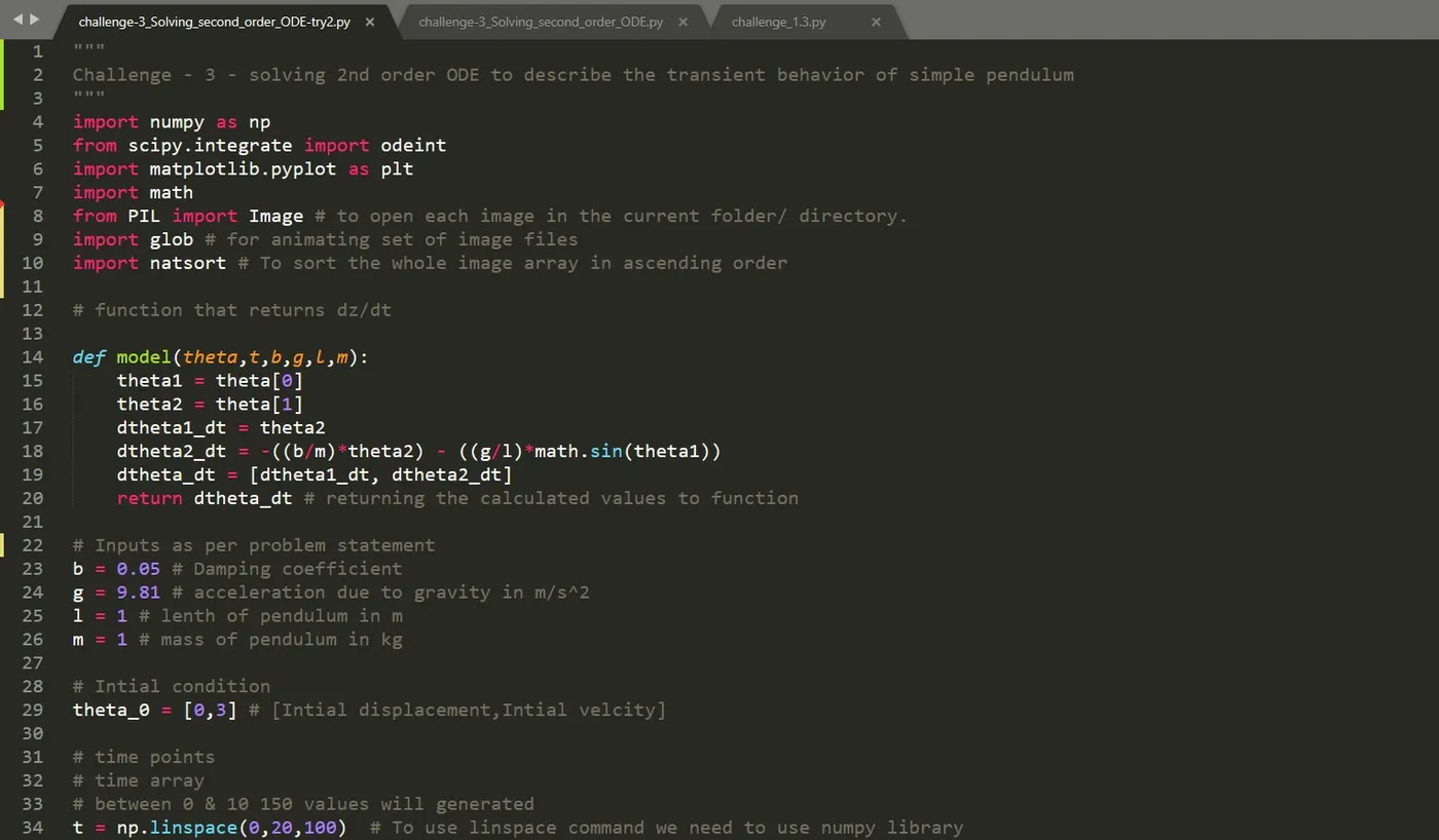
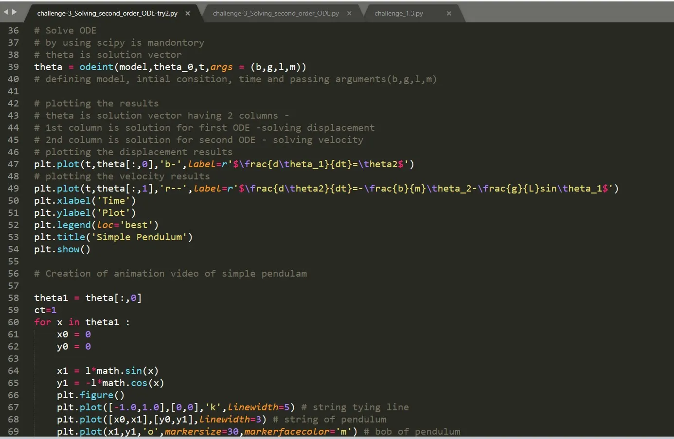
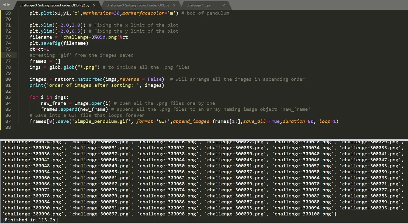
Code Explanation:

• The library module ‘math’ and ‘matplotlib.pyplot’ are imported using import command.
• The library module ‘PIL’ imported in order to open each image in the current folder/ directory.
• The library module ‘glob’ imported for animating set of image files,
• The library module ‘natsort’ imported to sort the whole image array in ascending order
• Defining 1st order ODE’s function derived by reducing the 2^nd order diff. equation of motion into 1^st order
• Passing input values Damping coefficient, acceleration due to gravity in m/s^2, length of pendulum in m and mass of pendulum in kg.
• Defining the initial condition for theta1 & theta2.
• Passing (t) for 20 sec and dividing it into 100 times.
• Solving ODE using odeint by calling defined ODE’s.
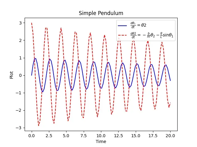
• Plotting Angular displacement and Velocity Vs Time with proper annotations, labels and titles
• To create an animation video, we need to retrieve the displacement of bob over time theta1 variables is assigned with displacement values
• Counter is introduced with initial value 1 for counting each frame.
• Using the for loop and counter ‘ct’, for the values of theta1 and theta 2 the coordinates of end of link1 to starting of link 2 and coordinates of end of link 2 to manipulator connecting point calculated for each of theta values
• Each of link positions with their respective coordinates are save as a ‘.png’ files
• ‘glob’ command is used to include all the100 (10*10 – 100) .png files for animation
• All the selected/included ‘.png’ files are sorted using the ‘natsort’ command and sorted files names are printed in display to verifying
• Inorder to animate all the 100 png files we create empty array called frames
• Using the for loop for each image, are opened and saved in empty array frames using ‘append’ command

Output:

Animation Video Link:

https://drive.google.com/file/d/16FECAn7h3Sv2MWys5f95xTTNjGcFzRrb/view?usp=sharing

Conclusion:

ODE represents the equation of motion of a simple pendulum with damping has been solved in python and we got position and velocity of pendulum with a function of time for 20sec. same has been used to create image in ‘.png’ format and all the ‘.png’ images are stitched to form the animation in GIF format