Week 3 - Solving second order ODEs

Objective

To setup the code for motion of Pendulum

Theory

The second order eqaution for simple pendulum is

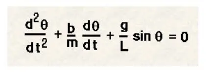
In given Equation

g = Gravity (m/s2) = 9.81

m= Mass of ball (kg) = 1

l = Length of the pendulum (m) = 1

b =Damping coefficient = 0.05

Simulate the motion between 0-20 sec, for angular displacement=0,angular velocity=3 rad/sec at time t=0.

Solving 2nd order ODE:

Assuming theta = theta1

diffrentiate dtheta_dt = dtheta1_dt = theta2

d^2theta_dt^2 = d^2theta1_dt^2 = dtheta2_dt

d^2theta_dt^2 + (b/m)dtheta_dt +(g/l)*sin(theta) = 0

d_theta2_dt + (b/m)theta2 +(g/l)sintheta1 = 0

dtheta1_dt = theta2

dtheta2_dt = -(b/m)*theta2 - (g/l)*sin(theta1)

Code

clear all
close all
clc

%Input parameters
l=1;
m=1;
b=0.05;
g=9.81;

%Initial Conditions
theta_0 = [0;3];

%Time points
t_span= linspace(0,20,500);

%Solve ODE
[t,results] = ode45(@(t,theta)ode_function(t,theta,b,g,l,m),t_span,theta_0);

%Plot the realtion of Angular displacement and Angular velocity
plot(t,results(:,1))

hold on
plot(t, results(:,2))
xlabel('time')
ylabel('Plot')
legend('Angular_displacement','Angular_velocity')
% To show the displacement results
displ=results(:,1);

%COde for pendulum
ct=1;

for i=1:length(t);
    
     %Initial position of the pendulum
     x0 = 0;
     y0 = 0;
     
     %Final position of the pendulum
     x1= l*sin(displ(i))
     y1= -l*cos(displ(i))
     
     %Plotting the second figure
     figure(2);
     
     %Base line
     plot([-1 1],[0 0], 'linewidth',3,'color','r')
     
     hold on
     
     %Pendulum string
     plot([x0 x1],[y0 y1],'linewidth',3,'color','r')
     
     %Pendulum Ball
     plot(x1,y1,'marker','o','markersize',25)
     
     %Axis fixing in plot
     axis([-2 2 -2 2])
     pause(0.02);
     
     hold off
     
     M(ct)= getframe(gcf);
     ct = ct+1;
     
end


movie(M);
videofile = VideoWriter('pendulum_oscillation.avi')
open(videofile);
writeVideo(videofile,M);
close(videofile);

Step Wise Explanation

%Input parameters
l=1;
m=1;
b=0.05;
g=9.81;

These are the paramters need to calculate the solution for the simple pendulum

theta_0 = [0;3];

In this theta_0 is assigned with initial angular displacement and angular velocity

Angular displacement = 0m

Angular velocity = 3m/sec

t_span= linspace(0,20,500);

Here the time span length is from 0 to 20 sec in between this range 500 values will be taken for the calculation

[t,results] = ode45(@(t,theta)ode_function(t,theta,b,g,l,m),t_span,theta_0);

To calculate θ1 and θ2 ‘ode 45’ command is used in MATLAB. By using ode45’ command, dθ1/dt` and dθ2/dt is solved to get angular displacement and angular velocity. Here 'results' is an array with 2 columns and rows equal to number of time values (here 500).

Ode45 is a function in matlab that solves ordinary or partial differential equations using a numerical method.

ode45(@(t,theta)ode_function : This is the Anonymous function in which function is defined in the name of ode_function

plot(t,results(:,1))
hold on
plot(t, results(:,2))
xlabel('time')
ylabel('Plot')
legend('Angular_displacement','Angular_velocity')

This command is used to plot the graph of Angular displacement and angular velocity

displ=results(:,1);

This command is used to show the displacement results, that is all the 1st coloumn values of displacement are shown. 500 values of displacement are shown in the results

%COde for pendulum
ct=1;

for i=1:length(t);

%Initial position of the pendulum
x0 = 0;
y0 = 0;

%Final position of the pendulum
x1= l*sin(displ(i))
y1= -l*cos(displ(i))

%Plotting the second figure
figure(2);

%Base line
plot([-1 1],[0 0], 'linewidth',3,'color','r')

hold on

%Pendulum string
plot([x0 x1],[y0 y1],'linewidth',3,'color','r')

%Pendulum Ball
plot(x1,y1,'marker','o','markersize',25)

%Axis fixing in plot
axis([-2 2 -2 2])
pause(0.02);

hold off

M(ct)= getframe(gcf);
ct = ct+1;

end

movie(M);
videofile = VideoWriter('pendulum_oscillation.avi')
open(videofile);
writeVideo(videofile,M);
close(videofile);

This command is used to plot the pendulum animation. In this initial position of pendulum is defined and the pendulum size and ball size is defined. Ball size is defined with the Marker

The values are calculated as loop with the help of for command. All the animation results are stored in the array defined by M

Code to call up the function

function[dtheta_dt] = ode_function(t,theta,b,g,l,m)

theta1= theta(1)
theta2= theta(2)
dtheta1_dt = theta2
dtheta2_dt = -(b/m)*theta2-(g/l)*sin(theta1);
dtheta_dt = [dtheta1_dt;dtheta2_dt];

end

Step Wise Explanation

In this function is defined with the name ode_function in which all the paraemters from the main program is called up in this function. The parameters are t,theta,b,g,l,m.

The second order Differential equation is solved into 1 st order DE in order to calculate the values of theta 1 and theta 2 .

2 terms are stored in dtheta1_dt and dtheta2_dt. This values are going to be stored inside dtheta_dt in which this values are going to transfer in the main program.

Results

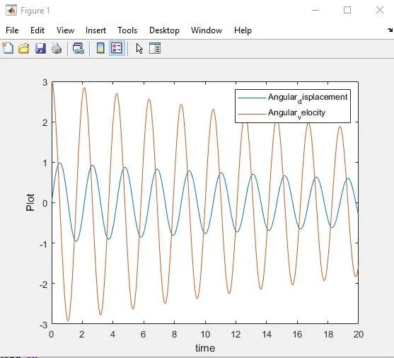
The pendulum oscillation and graph is plotted for Angular displacement and Angular velocity from the above code

Error while coding

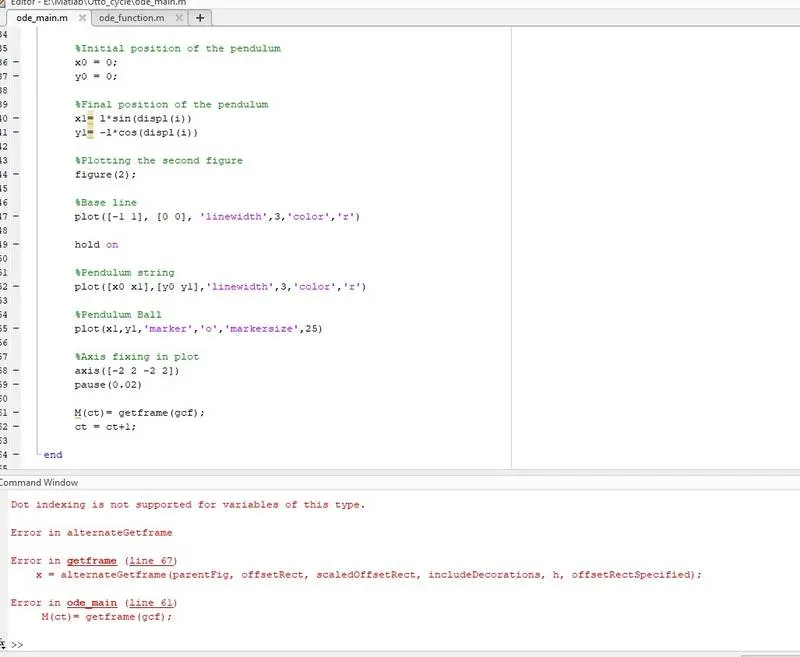
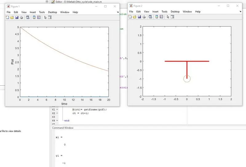
Due to the above error the results obtained frm the code is shown below

This error is because of in the function one of the code is wriiten as "dtheta1_dt = theta1".

Actually the code should be "dtheta1_dt = theta2"

After replacing the theta1 by theta2 correct results obtained.

Conclusion

Governing differential equation of simple pendulum is solved using MATLAB program. Animation is working correctly. Hence it can be concluded that solution obtained by program is correct.