Week 3 - Solving second order ODEs

Aim : To solve second order ODE's in matlab.

Objective: To write a program to solve second order ode's and plot the graph in

the matlab and to create an animation to stimulate the pendulum motion.

Equations :

`(d^2θ)/(dt^2)+b/m*(dθ)/dt+g/lsinθ=0`

`theta = theta_1`

`(d theta)/dt=(d theta_1)/dt=theta_2`

`(d^2 theta)/dt=(d^2 theta_1)/dt^2=d/dt((d theta_1)/dt)=d/dt(theta_2)`

`(d^2 theta)/dt^2+b/m.(d theta_1)/dt=g/lsin theta=0`

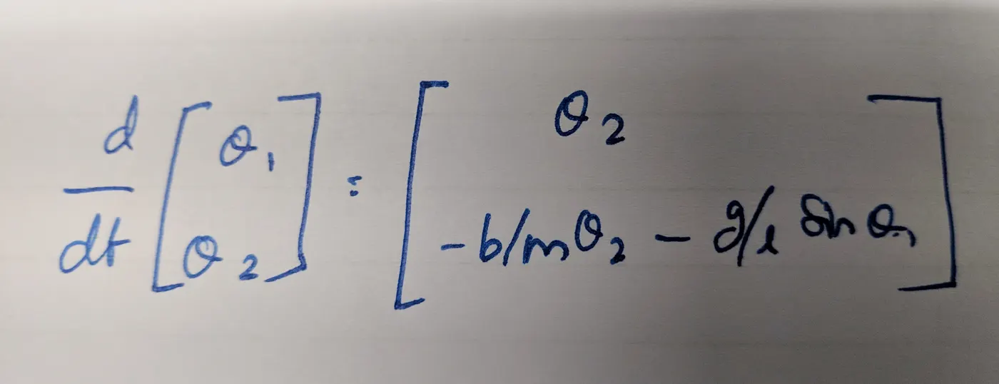
`(d theta_1)/dt+b/m theta_2+g/lsin theta_1=0`

`(d theta_1)/dt=theta_2`

`(d theta_2)/dt=-b/mtheta_2-g/lsin theta_1`

where as,

g= gravity

m = mass

l = length

b = damping coefficient

Inputs:

Length l=1 metre,

Mass m=1 kg,

Damping coefficient b=0.05,

gravity g=9.81 m/s^2,

Diplacement= 0,

Angular velocity=3,

Time span=0-20 sec,

Time t=0,

b=0.05;
g=9.81;
l=1;
m=1;

%initial conditions:

theta_0 = [0;3];

%time points

t_span = linspace(0,20,500);

By giving the above commands we have givrn the inputs and initial conditions.

Solution for ODE :

function
[dtheta_dt] = ode_func(t,theta,b,g,l,m)
theta1 = theta(1);
theta2 = theta(2);
dtheta1_dt = theta2;
dtheta2_dt = -(b/m)*theta2 - (g/l)*sin(theta1);
dtheta_dt = [dtheta1_dt;dtheta2_dt];
end

function command is created where the 3rd order ode is breaked down into two simple

2nd order ode.

% solve ode

[t, results] = ode45(@(t,theta) ode_func(t,theta,b,g,l,m),t_span,theta_0);
hold on
subplot(2,1,1)
plot(t,results(:,1),'linewidth',3,'color','y')
xlabel('time')
ylabel('displacement')
grid on
subplot(2,1,2)
plot(t,results(:,2),'linewidth',3,'color','b')
xlabel('time')
ylabel('angular velocity')
grid on

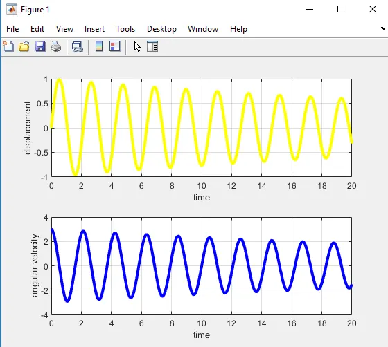
ode 45 is a solver which is used instead of for loop to make the command less

complicated.

In the ode 45 function , intergal limits, and initial conditions are given.

the fuction command is called using after ode45.

Sub plot command is used to plot in two different graphs. hold on & hold off command

is used to plot the second graph without deleting the first plot.label command is used to

label the x and y axis in the graph. grid on commands is used to turn on the grids in the

graph.

Animation of pendulum:

%pendulum:


ct = 1;
coordinate = results(:,1)

for i = 1:length(coordinate)
    THETA = coordinate(i);   
    
    x_1 = 0;
    y_1 = 0;
    
    x_2 = 1*sin(THETA);
    y_2 = -l*cos(THETA);
  figure(2)
  
    plot([x_1 x_2],[y_1 y_2],'linewidth',3,'color','b')
    line([-1   1],[0 0],'linewidth',5,'color','b')
    hold on
  plot(x_2,y_2,'marker','o','markersize',40,'markerfacecolor','r')
  hold off
    axis([-1.5 1.5 -1.2 .2])
    M(ct) = getframe(gcf)
    ct = ct+1;
    
   
end

Coordinates is values in the 1st column of the results from the ode45 solver. where

the i is equal to the 1 tpo length of the values from ode45 solution. where THETA

is equal to the coordinates of i. x_1 , y_1 is the fixed point so the values of the

both remains constant.x_2 and y_2 is moving end of the pendulum. x_2 is equal to

l *sin (ThETA) where THETA is the value which we get from the ode45 which

automatically iterarte itsef according to the limits and the values given.

same as with the y_2 where y_2 is equal to -1*cos(THETA). then these values

obtained are plotted using the plot command. line of axiss where the fixed point of

pendulum is located is created using line command. axis command is used to define

the area limit where the pendulum moves .

close all
clear all
clc

b=0.05;
g=9.81;
l=1;
m=1;

%initial conditions:

theta_0 = [0;3];

%time points

t_span = linspace(0,20,500);

% solve ode

[t, results] = ode45(@(t,theta) ode_func(t,theta,b,g,l,m),t_span,theta_0);
hold on
subplot(2,1,1)
plot(t,results(:,1),'linewidth',3,'color','y')
xlabel('time')
ylabel('displacement')
grid on
subplot(2,1,2)
plot(t,results(:,2),'linewidth',3,'color','b')
xlabel('time')
ylabel('angular velocity')
grid on

%pendulum:


ct = 1;
coordinate = results(:,1)

for i = 1:length(coordinate)
    THETA = coordinate(i);   
    
    x_1 = 0;
    y_1 = 0;
    
    x_2 = 1*sin(THETA);
    y_2 = -l*cos(THETA);
  figure(2)
  
    plot([x_1 x_2],[y_1 y_2],'linewidth',3,'color','b')
    line([-1   1],[0 0],'linewidth',5,'color','b')
    hold on
  plot(x_2,y_2,'marker','o','markersize',40,'markerfacecolor','r')
  hold off
    axis([-1.5 1.5 -1.2 .2])
    M(ct) = getframe(gcf)
    ct = ct+1;
    
   
end
movie(M)
videofile = VideoWriter('pendulum_motion.avi','uncompressed avi');
open(videofile)
writeVideo(videofile,M)
close(videofile)
    

Conclusion:

Thus the command to solve the ode and to generate the animation for the motion of

the pendulum is done.

Click here for the link for the matlab save file.