Week 3 - Solving second order ODEs
WEEK 3 - SOLVING SECOND ORDER ODES
ABSTARCT
This report is about generation of animation for the simple pendulum swing and applying ordinary differential equation(ODE) to solve simple pendulum equation of motion. Furthermore, usage of functions like ‘ode45’, anonymous function and ‘makers’ and their syntax. The step-by-step code generation in MATLAB and logic is explained and errors appeared during process of successful execution of code and steps are taken to resolve them. Additionally, evidence of errors is documented in the report. The YouTube link is provided for animation.
THEORY
The following paragraphs will delineate about the brief theory and basic concept and logic of the MATLAB functions used in this report for generating the simple pendulum oscillation animation files and plots.
The ordinary differential equations (ODE) are essential in solving several analytical mechanics when a problem is involved with dependent and independent variables with derivatives. The ODE is nothing, but which consist of one or more functions of one independent variable and derivative of those functions. In contrast, the partial differential equation consists of more than one independent variable.
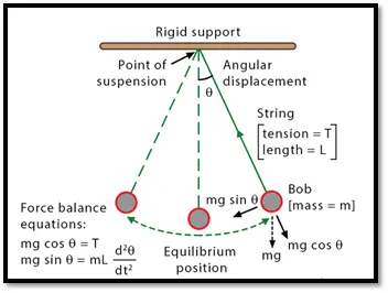
The simple pendulum is one which has bob with certain mass(m), is attached to string of length(L) and is attached to a rigid structure. Pendulum oscillated when small amount of displacement is given with certain initial angle, then it oscillates with periodic motion. The oscillations are dampened due to damping factor. The oscillation of simple pendulum is considered to be simple harmonic oscillation. The following figure depicts simple pendulum.
The following is the equation of motion for simple pendulum:
Equation 1:
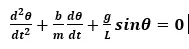
b= Damping coefficient
m= Mass of the bob in kg
g= Acceleration due to gravity in m/s^2
L= length of string in m
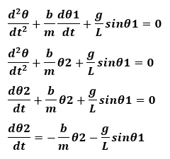
For coding in MATLAB, I use the function ‘ode45’ which works based on simple numerical method and 4th order Runge Kutta method, for that reason, I have break second order ODE in to first order ODE. The ‘ode45’ works with first order ODE. Now in the following, I would be breaking down the 2nd order ODE into 1st order ODE.
Now,
θ= θ1
so, the equation 1 becomes Equation 2:
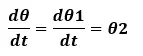
Equation 3:
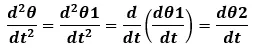
By substituting equation 2 and equation 3 into equation 1, the equation becomes
The vector form of the variables is in matrix form:
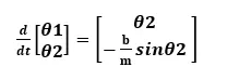
Function ‘ode45’, is unique built in function in MATLAB, it takes three inputs: first one is functioned to be integrated, second one is time span and final one is initial conditions. The integration limits are time span and it is provided as vector of 2 values, that is initial and final time limits are created with ‘linspace’ function. The initial condition is the function of time at t=0.
Anonymous function: it is new function which is utilized in this code. Unlike any other function, these are not stored as separate files. These don’t have any starting ‘function’ and ‘end’ handles. This kind of functions handles are declared in main MATLAB code, and they accessible and localized to particular condition.
Function handle declaration is similar to function declaration. This is observed with ‘@’ symbol before the input arguments.
The syntax is : Funct_handle=@(input_argu) function_def
here, Funct_handle is the name of the particular handle
Input argument is the one which will be fed into the function
function_def will have the equation/expression which will use the input to give us the output. The syntax for calling this particular function handle is
Var_name=Funct_handle(input_argu)
So, the output from the handle will be stored under ’Var_name’
MATLAB CODE STEP-BY-STEP DESCRIPTION
The code below is without comments but in the following paragraphs, code is explained elaborately. The main code file “Air_Standard_Cycle_Call_By_Function_1.m” with comments is uploaded to the SKILL-LYNC site.
clear all
close all
clc
b=0.05
g=9.81
l=1
m=0.1
theta_0=[0;3]
time_span=linspace(0,20,500)
[t,outputs]=ode45(@(t,theta) ode_funct(t,theta,b,g,l,m),time_span,theta_0);
figure(1)
plot(t,outputs(:,1),'linewidth',3,'color','c')
title('ANGULAR DISPLACEMNT & ANGULAR VELOCITY with respective to Time')
hold on
plot(t,outputs(:,2),'linewidth',3,'color','m')
axis([0 11 -5 5])
grid on
legend('ANGULAR VELOCITY','DISPLACEMNT')
ylabel('ANGULAR VELOCITY & DISPALCEMNT')
xlabel('TIME in SEC')
figure(2)
plot(outputs(:,1),outputs(:,2))
grid on
xlabel('POSITION in RADIANS')
ylabel('ANGULAR VELOCITY in rad/sec')
title('ANGULAR VELOCITY vs ANGULAR DISPLACEMNT')
theta2=outputs(:,1)
count=1
for dis=1:length(theta2)
theta3=theta2(dis)
x0=0;
y0=0;
x1=1*sin(theta3)
y1=-1*cos(theta3)
figure(3)
plot([-1.1 1.1],[0 0],'linewidth',4)
hold on
plot([x0 x1],[y0 y1],'color','g','linewidth',4)
hold on
plot(x1,y1,'o','markers',22,'markerfacecolor','r')
title('PENDULUM ANIMATION')
hold off
grid on
axis([-1.5 1.5 -1.5 0.5])
pause(0.03)
M(count)=getframe(gcf)
count=count+1
end
movie(M)
videofile=VideoWriter('Pendulum.avi','uncompressed avi')
open(videofile)
writeVideo(videofile,M)
close(videofile)
The above main code consists of a function which is mainly for solving second order differential equation. From this function, the outputs of dtheta2_dt and dtheta2_dt are stored in an array with separator, so that they will be two column matrixes. first column is for angular displacement and second column is for angular velocity.
The functions can be called in to any MATLAB main file code, by calling appropriate parameters in right order to meet correct execution of the program. The functions are tested before they are actually called in the main code and we need not run the entire main file, so it is advantageous for creating functions.
The main function code file with comments is “ode_funct.m” uploaded to SKILL-LYNC website. The following is the function code without comments. Here I am defining theta1 and theta2, is solution array. This is first order ordinary differential equation “dtheta1_dt=theta2” and It is second order ODE :”dtheta2_dt=-(b/m)*theta2-(g/1)*sin(theta1)”.
From this function, the outputs of dtheta2_dt and dtheta2_dt are stored in an array with separator, so that they will be two column matrixes. First column is for angular displacement and second column is for angular velocity.
function[dtheta_dt]=ode_funct(t,theta,b,g,l,m)
theta1=theta(1)
theta2=theta(2)
dtheta1_dt=theta2
dtheta2_dt=-(b/m)*theta2-(g/1)*sin(theta1)
dtheta_dt=[dtheta1_dt;dtheta2_dt]
end
Here, the MATLAB code which consist of series of functions are explained in detailed. Firstly, there are three functions used in the MATLAB to clear previous functions int the function, results and result plots. They are:
'clear all': This function removes all variables, functions and MEX-files from-memory and leaving workspace empty.
'close all': This function will close all the figure handles are visible and hidden figure handles
'clc': function clears text from function window.
Secondly, the following are the initial variables in the simple pendulum equation of motion.
b= Damping coefficient
m= Mass of the pendulum bob in kg
g= Acceleration due to gravity m/s^2
l= Length of string in meters or m
b=0.05
g=9.81
l=1
m=0.1
At starting, the initial conditions for ‘theta_0’ for solving differential equation are provided: initial angular displacement and initial angular velocity.
theta_0=[0;3]
The time span 0 to 20 seconds and obtaining 500 equal intervals from 'linspace' function, which is used to provide time limits and equal intervals. Time span is the time for rotation of the simple pendulum.
time_span=linspace(0,20,500)
Now, Solving ODE through inbuilt function ‘ode45’: is in-built solver in MATLAB. Main inputs are theta and t are dependent and independent variables of the system. Here, we are defining function consist of parameters t, theta, b,g,l,m,t_span, theta_0. Provide time_span which is time array for integration points and theta_0 as initial conditions.
First, define ODE as Anonymous function of t, theta, Second, the ‘ode_funct’ function is defined with all the parameters. This function solves second order ODE in function file which is called here. The ode_funct is called along with anonymous function, time_span and theta_0
Finally, the function gives me integration ‘time’ and ‘outputs’. The outputs will have two columns :First column for angular displacement and second column consist of angular velocity.
[t,outputs]=ode45(@(t,theta) ode_funct(t,theta,b,g,l,m),time_span,theta_0);
The 'figure' function is used for creating a window for plotting all the state points. The 'hold on' function retains the current plot and certain axes properties so that subsequent graphing commands add to the existing graph. The 'plot' function is used for plotting the angular velocity and angular displacement Vs time. The 'hold on' function is utilized for plotting angular displacement and angular velocity in one plot against time. The 'title' function will help in providing heading to the plot. The 'xlabel' function will help in giving name to x-axis .The 'ylabel' function will help in giving name to y-axis. The 'legend' function places a legend on various types of graphs (line plots, bar graphs, pie charts, etc.). For each line plotted, the legend shows a sample of the line type, marker symbol, and color beside the text label you specify.
figure(1)
plot(t,outputs(:,1),'linewidth',3,'color','c')
title('ANGULAR DISPLACEMNT & ANGULAR VELOCITY with respective to Time')
hold on
plot(t,outputs(:,2),'linewidth',3,'color','m')
axis([0 11 -5 5])
legend('ANGULAR VELOCITY','DISPLACEMNT')
ylabel('ANGULAR VELOCITY & DISPALCEMNT')
xlabel('TIME in SEC')
figure(2)
plot(outputs(:,1),outputs(:,2))
xlabel('POSITION in RADIANS')
ylabel('ANGULAR VELOCITY in rad/sec')
title('ANGULAR VELOCITY vs ANGULAR DISPLACEMNT')
The following code is for creating of no of images of pendulum swing and finally storing it in the video format, so I have 'count' variable and 'theta2'. The 'count variable is used count number of events inside the for loop and to count the no frames of pendulum images are taken.
theta2=outputs(:,1)
count=1
The following 'for' loop is for capturing the moving end of pendulum and recording the movie with help of array of pictures. The x0,y0 are coordinates of fixed end of the pendulum. The 'figure' function is creating new window for the animation. The 'figure' function is creating new window for the animation. The 'plot' function is creating a rigid horizontal line for pendulum to be fixed at on a point. The 'hold on' function is for accommodating other plots. The 'plot' function is plotting pendulum arm for start and final state. Now, x1 and y1 is an array of 500 values. it has line width 4 and color green. The 'hold on' function is for accommodating other plots.
The 'plot' function is used for marking pendulum bob and used 'markers' function for shape of the bob, size of bob and color of the bob. The 'title' function will help in providing heading to the plot as “PENDULUM ANIMATION”. the 'axis' function is used for defining the axes limits. The 'pause' function is used for pausing the frame 0.03 seconds between two consecutives frame. All the frames stored in the M, the function 'getframe(gcf) takes array of frames. The counter is iterated. Finally, ‘for’ loop ends.
for dis=1:length(theta2)
theta3=theta2(dis)
x0=0;
y0=0;
x1=1*sin(theta3)
y1=-1*cos(theta3)
figure(3)
plot([-1.1 1.1],[0 0],'linewidth',4)
hold on
plot([x0 x1],[y0 y1],'color','g','linewidth',4)
hold on
plot(x1,y1,'o','markers',22,'markerfacecolor','r')
title('PENDULUM ANIMATION')
hold off
grid on
axis([-1.5 1.5 -1.5 0.5])
pause(0.03)
M(count)=getframe(gcf)
count=count+1
end
At this point of time, the function movie(M)' will help in playing the movie in matrix form once.
movie(M)
The 'VideoWriter()' function will create an object to write video file from an array or MATLAB Movie. This object has info about video and properties that control output video. here I am writing video file into "avi" format and uncompressing the video. the video is written to videofile.
videofile=VideoWriter('PendulumP.avi','Uncompressed AVI')
The'open' function is helpful in opening specified file or variable in appropriate application.
open(videofile)
The 'writeVideo' function is used to writes data from an array to the video file associated with name of the file.
writeVideo(videofile,M)
The 'close' function is used to close the video file.
close(videofile)
ERORS FACED AND STEPS TO OVERCOME
The following paragraphs will illustrate various errors encountered during programing and steps taken to resolve.
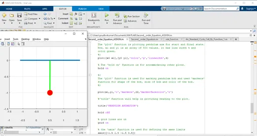
- The below screenshot shows a syntax error for providing axes limits through ‘axis function.
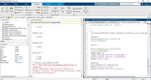
From the command window of MATLAB, the error is emphasized at line number 71. Now by providing “( )” around axis ([0 25 -3 3], the issue is resolved. The below figure depicts it.
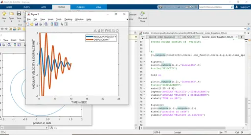
The other trouble is fixing plot within the window frame, it is fixed by putting appropriate axis limits from the output values. The following pic talks about it.
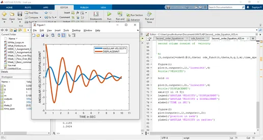
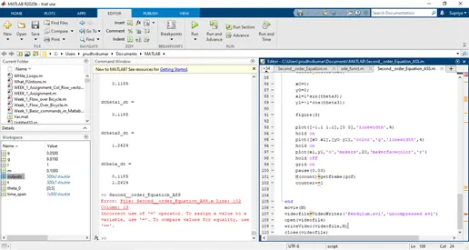
2. In this scenario, I incremented the “counter+=1” in the wrong way, so MATLAB threw an error saying wrong use of “=” operator. The follows screenshot exhibit that.
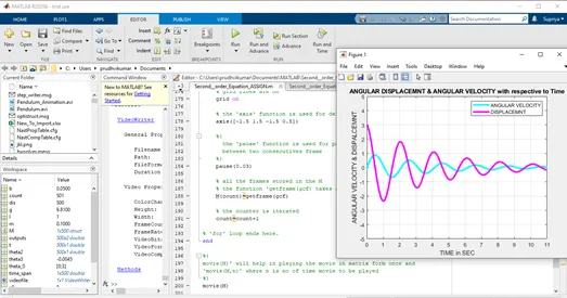
The issue was resolved by correct use of counter increment “counter=counter+1”. The below picture is evidence for solving the error.
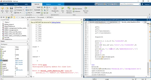
3. The other error occurred due to typo mistake, that is, for ‘markers’, I mentioned it as ‘makers’. The MATLAB shown error. The following is screenshot that shows error.
The mistake is resolved by following MATHWORKS library for correct spelling for ‘markers’. The below screenshot will show.
OUTPUT
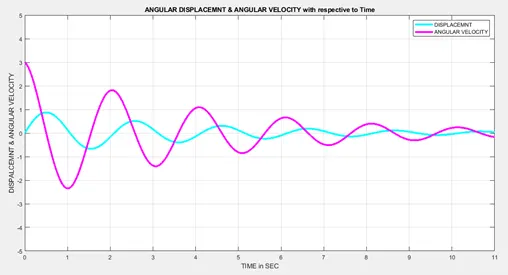
After breaking down the second order ODE into first order ODE, with application of ‘ode45’ function and anonymous function, from output, plots for Angular displacement and Angular velocity Vs time is plotted. As , the damping coefficient b=0.05, we can observe the oscillation coming to still within 11 seconds. The below is the plot:
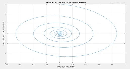
The following other output plot for the Angular velocity against angular displacement.
The final simple pendulum oscillation animation is uploaded to YouTube: https://youtu.be/BZVxiSH-7Sk
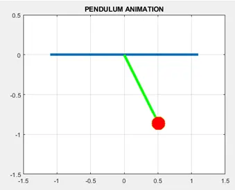
The below is picture of the pendulum oscillation. Finally, pendulum displacement with respective time is created.
References:
- The lecture videos
- Simple pendulum picture: https://www.sciencefacts.net/simple-pendulum.html
- https://www.acs.psu.edu/drussell/Demos/Pendulum/Pendula.html
- https://en.wikipedia.org/wiki/Pendulum_(mathematics)
- https://courses.lumenlearning.com/physics/chapter/16-4-the-simple-pendulum/
- https://web.njit.edu/~kenahn/11spring/phys106/Lecture/L23.pdf
- https://www.acs.psu.edu/drussell/Demos/Pendulum/Pendulum.html#:~:text=By%20applying%20Newton's%20secont%20law,enough%2C%20so%20the%20small%20angle
- https://www.sciencefacts.net/simple-pendulum.html
%{
Creation of Simple Pendulum animation using equation of motion
for simple pendulum with application of Ordinary Differential Equation
 %}


%{
'clear all' function removes all the variables, functions and MEX-files
from-memory and leaving workspace empty.

'close all' function will closes all the figure handles are visible and
 hidden figure handles.

 'clc' function clears text from command window.
%}
clear all
close all
clc


%{
the following are the initial variables in the simple pendulum
equation of motion.
b= Damping coefficient
m= Mass of the pendulum bob in kg
g= Acceleration due to gravity m/s^2
l= Length of string in meters or m

%}

b=0.05
g=9.81
l=1
m=0.1

%{
At starting, the initial conditions for theta for solving differential
equation are provided: initial angular displacement and
initial angular velocity.

%}

theta_0=[0;3]

%{
The time span 0 to 20 seconds and obtaining 500 equal intervals
from 'linspace' function, which is used to provide time limits and
equal intervals. Time span is the time for rotation of the simple pendulum.

%}
time_span=linspace(0,20,500)

%{
Solving ODE through inbuilt function

ode45: is in-built solver in MATLAB

Now, Solving ODE through inbuilt function ‘ode45’: is in-built solver
in MATLAB. Main inputs are theta and t are dependent and independent
variables of the system. Here, we are defining function consist of
parameters t, theta, b,g,l,m,t_span, theta_0.
Provide time_span which is time array for integration points and
theta_0 as initial conditions.First, define ODE as Anonymous function of t,
theta, Second, the ‘ode_funct’ function is defined with all the parameters.
This function solves second order ODE in function file which is called
here. The ode_funct is called along with  anonymous function,
time_span and theta_0. Finally, the function gives me integration ‘time’
and ‘outputs’. The outputs will have two columns :First column  for
angular displacement and second column consist of  angular velocity.

%}
[t,outputs]=ode45(@(t,theta) ode_funct(t,theta,b,g,l,m),time_span,theta_0);

%{
'figure' function is used for creating a window for plotting
all the state points

'hold on' function retains the current plot and certain axes properties so
that subsequent graphing commands add to the existing graph

'plot' function is used for plotting the velocity and displacement Vs time.
 'hold on' function is utilized for ploting angular displacement and
 angular velocity in one plot against time.
'title' function will help in providing heading to the plot.
'xlabel' function will help in giving name to x-axis
'ylabel' function will help in giving name to y-axis
'legend' function places a legend on various types of graphs
(line plots, bar graphs, pie charts, etc.). For each line plotted,
 the legend shows a sample of the line type, marker symbol, and color
beside the text label you specify.
%}

figure(1)

plot(t,outputs(:,1),'linewidth',3,'color','c')
title('ANGULAR DISPLACEMNT & ANGULAR VELOCITY with respective to Time')
hold on
plot(t,outputs(:,2),'linewidth',3,'color','m')
axis([0 11 -5 5])
% grid lines are on
grid on
legend('DISPLACEMNT','ANGULAR VELOCITY')
ylabel('DISPALCEMNT & ANGULAR VELOCITY')
xlabel('TIME in SEC')

figure(2)
plot(outputs(:,1),outputs(:,2))
% grid lines are on
grid on
xlabel('POSITION in RADIANS')
ylabel('ANGULAR VELOCITY in rad/sec')
title('ANGULAR VELOCITY vs ANGULAR DISPLACEMNT')


%{
the following code is for creating of no of images of pendulum swing and
finally storing it in the video format, so i have 'count' variable and
'theta2'.

the 'count variable is used count number of events inside the for loop and
to count the no frames of pendulum images are taken.
%}
theta2=outputs(:,1)
count=1

%{
The following 'for' loop is for capturing the moving end of pendulum and
recording the movie with help of array of pictures.
%}
for dis=1:length(theta2)
    theta3=theta2(dis)
   % the x0,y0 are fixed end of the pendulum
    x0=0;
    y0=0;
    x1=1*sin(theta3)
    y1=-1*cos(theta3)

    % 'figure' function is creating new window for the animation
    figure(3)

    %{
    The 'plot' function is creating a rigid horizontal line for pendulum
    to be fixed at on a point.
    %}
    plot([-1.1 1.1],[0 0],'linewidth',4)

    %The 'hold on' function is for accommodating other plots.

    hold on

    %{
    The 'plot' function is plotting pendulum arm for start and final state.
    Now, x1 and y1 is an array of 500 values. it has line width 4 and
    color green.
    %}
    plot([x0 x1],[y0 y1],'color','g','linewidth',4)

     % the 'axis' function is used for defining the axes limits
    axis([-1.5 1.5 -1.5 0.5])

    % The 'hold on' function is for accommodating other plots.
    hold on


    %{
    The 'plot' function is used for marking pendulum bob and used 'markers'
    function for shape of the bob, size of bob and color of the bob.
    %}

    plot(x1,y1,'o','markers',22,'markerfacecolor','r')

    %'title' function will help in providing heading to the plot.

    title('PENDULUM ANIMATION')

    hold off

    % grid lines are on
    grid on

    %{
      the 'pause' function is used for pausing the frame 0.03 seconds
      between two consecutives frame
    %}
    pause(0.03)

    % all the frames stored in the M
    % the function 'getframe(gcf) takes array of frames
    M(count)=getframe(gcf)

    % the counter is iterated
    count=count+1

% 'for' loop ends here.
end

%{
movie(M)' will help in playing the movie in matrix form once and
'movie(M,n)' where n is no of time movie to be played
%}
movie(M)

%{
'VideoWriter()' function will create an object to write video file
from an array or MATLAB Movie. this object has info about video and
properties that control output video. here I am writing video file
into "avi" format and uncompressing the video. the video is written
to videofile.
%}
videofile=VideoWriter('PendulumP.avi','Uncompressed AVI')

%{
'open' function is helpful in opening specified file or variable
in appropriate application
%}
open(videofile)

%{
'writeVideo' function is used to writes data from an array to the
video file associated with name of the file.
%}
writeVideo(videofile,M)

%'close'used to close the video file.
close(videofile)


% the following is the function

%{
this function is mainly for solving second order differential equation.
%}

function[dtheta_dt]=ode_funct(t,theta,b,g,l,m)

%{
Here I am defining theta1 and theta2, is solution array
%}

theta1=theta(1)
theta2=theta(2)

%the below is first order ordinary differential equation

dtheta1_dt=theta2

%It is second order ODE

dtheta2_dt=-(b/m)*theta2-(g/1)*sin(theta1)

%{
From this function, the outputs of dtheta2_dt and dtheta2_dt are stored
in an array with separator, so that they will be two column matrixes.
first column is for angular displacement and second column is
for angular velocity.
%}
dtheta_dt=[dtheta1_dt;dtheta2_dt]


end