Week 3 - Solving second order ODEs
AIM
To wite a program in Matlab\Octave that will simulate the pendulum motion by solving the ODE.
OBJECTIVE
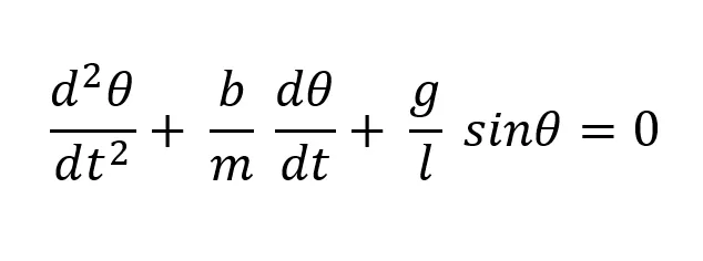
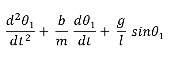
Your objective is to write a program that solves the following ODE. This ODE represents the equation of motion of a simple pendulum with damping
THEORY/ DESCRIPTION
A Pendulum is a body suspended from a fixed support so that it swings freely back and forth under the influence of gravity. When a pendulum is displaced sideways from its resting, equilibrium position, it is subject to a restoring force due to gravity that will accelerate it back toward the equilibrium position. When released, the restoring force acting on the pendulum's mass causes it to oscillate about the equilibrium position, swinging it back and forth. The mathematics of pendulums are in general quite complicated. Simplifying assumptions can be made, which in the case of a simple pendulum allow the equations of motion to be solved analytically for small-angle oscillations.
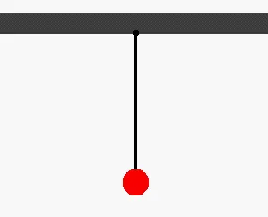
ODEs are extremely important in engineering, they describe a lot of phenomenon and solving those ODEs can help us understand the steps. Simple Pendulum is an perfect example that involves the Second order differetial equation. In solving equation for pendulum we are solving for the theta and the rate at which the theta value changing with respect to time which is known as velocity. In addition to this the same pendulum describe the motion of a spring, mass and a damper system.This has a lot of application in vehicle dynamics.
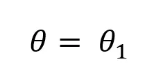
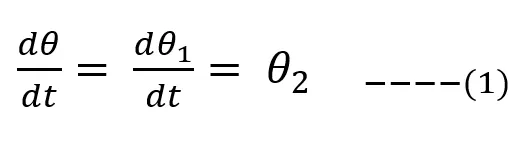
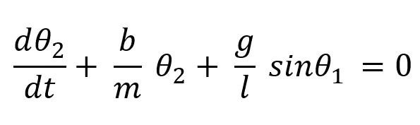
The fundamental idea behind solving ODEs both analytical and computational is breaking down the higher order ODE into set of first order ODE. So here the equation is second order differential equation.
If,
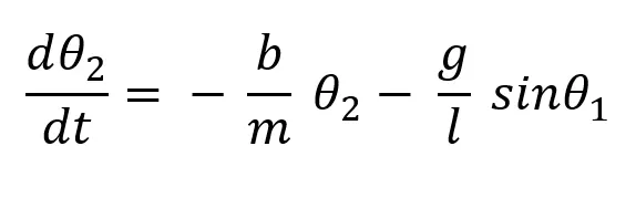
then,

Back to original ODE,
In the above equation,
g = gravity in m/s2,
L = length of the pendulum in m,
m = mass of the ball in kg,
b=damping coefficient.
Thus our second order differential equation is broke down into series of first order differential equation.
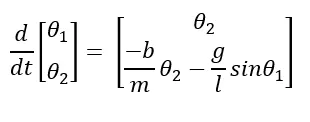
Here, d/dt = (θ1/θ2) is taken as θ.
PROGRAM EXPLANATION
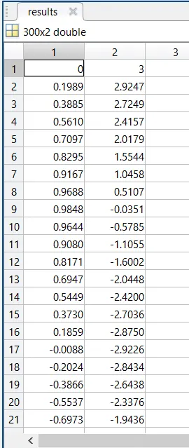
First all the parameters were given as inputs such as damping coefficient, gravity, length of the pendulum, mass of the ball. And the initial conditions were given as initial displacement is given as 0 and initial velocity is given as 3 rad/sec. Then time is allocated in array. And next here ode45 is a inbuilt function here. Ode45 is a function in matlab that solves ordinary or partial differential equations using a numerical method.
To solve an ODE, we have to integrate and solve for the variable. Assuming we have an ode du, we would solve for u by integrating du provided some limits of integration. However, rather than direct integration, we can use a numerical solver, by discretising the equation, that is, we convert the ODE into a linear equation and then solve this equation to approximate the solution. The function can be provided in the form of an anonymous function,
[t,y] = ode45(odefun,tspan,y0) ,odefun is a function program.
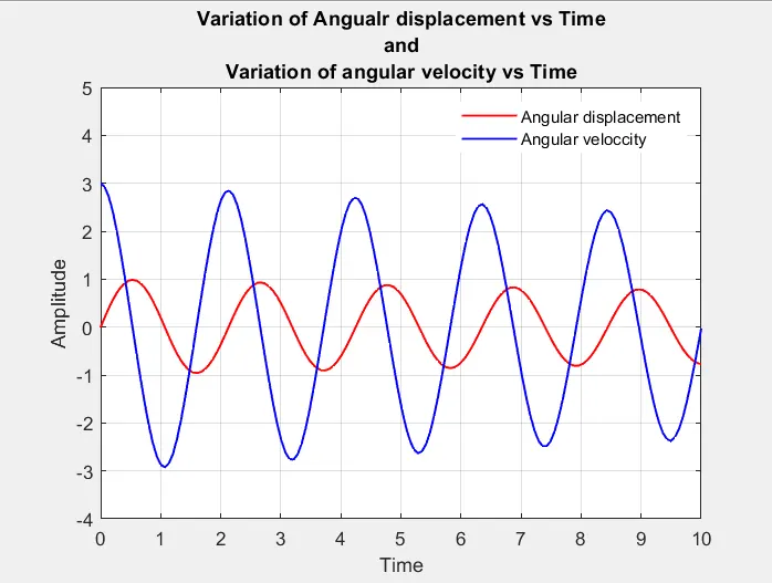
Here comes the first code for plotting graph betwwen the varying angular displacement and velocith with regards to time.
MATLAB CODE
clear all
close all
clc

b=0.05;  %damping coefficient
g=9.81;  %gravity
l=1;     %length of the pendulum
m=1;     %mass of the ball

%initial condition
theta_0 = [0;3];

%time points
t_span = linspace(0,20,300);

%solve ODE
[t,results] = ode45(@(t,theta)ode_func(t,theta,b,g,l,m),t_span, theta_0);

figure(1) %Graph
plot(t,results(:,1),'linewidth',1,'color','r'); %Plotting angular disp vs time
hold on;
plot(t,results(:,2),'linewidth',1,'color','b'); %Plotting angular velocity vs time
xlabel('Time');
ylabel('Amplitude');
title({'Variation of Angualr displacement vs Time','and','Variation of angular velocity vs Time'});
legend('Angular displacement','Angular veloccity');
axis([0 10 -4 5]);
grid on
MATLAB CODE
odefunc program is attached below where the theta calculation is done.
function [dtheta_dt] = ode_func(t,theta,b,g,l,m)

theta1 = theta(1)
theta2 = theta(2)
dtheta1_dt = theta2;
dtheta2_dt = -(b/m)*theta2 - (g/l)*sin(theta1);
dtheta_dt = [dtheta1_dt; dtheta2_dt];
end
This is calculated in the odefunc program and been called in the main program.
VARYING ANGULAR DISPLACEMENT AND VARYING ANGULAR VELOCITY WITH RESPECT TO TIME
GRAPH
VARYING ANGULAR DISPLACEMENT AND VARYING ANGULAR VELOCITY
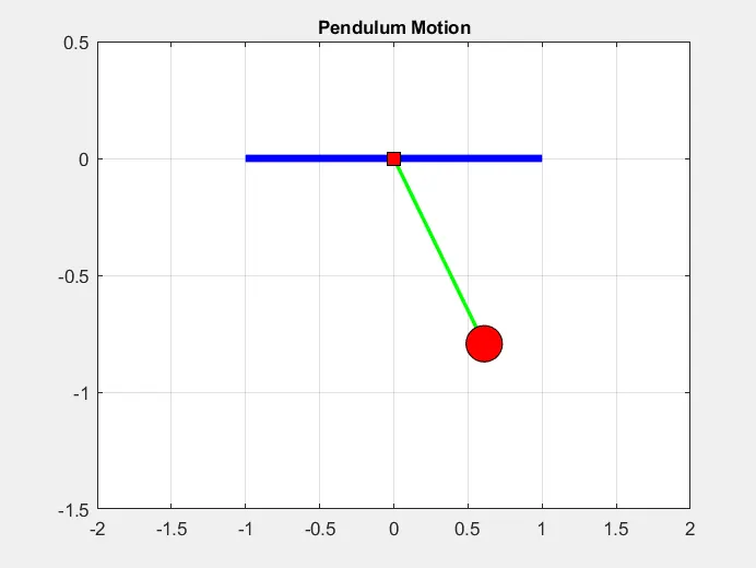
Now the program for animating the pendulum motion in Matlab is generated using marker command circle for ball and the marker command square for the pivot.
MATLAB CODE
clear all
close all
clc

b=0.05;  %damping coefficient
g=9.81;  %gravity
l=1;     %length of the pendulum
m=1;     %mass of the ball

%initial condition
theta_0 = [0;3];

%time points
t_span = linspace(0,20,300);

%solve ODE
[t,results] = ode45(@(t,theta)ode_func(t,theta,b,g,l,m),t_span, theta_0);

figure(1) %Graph
plot(t,results(:,1),'linewidth',1,'color','r'); %Plotting angular disp vs time
hold on;
plot(t,results(:,2),'linewidth',1,'color','b'); %Plotting angular velocity vs time
xlabel('Time');
ylabel('Amplitude');
title({'Variation of Angualr displacement vs Time','and','Variation of angular velocity vs Time'});
legend('Angular displacement','Angular veloccity');
axis([0 10 -4 5]);
grid on

figure(2) %Pendulum motion
ct=1;

for i=1:length(results(:,1))
    x0=0;
    y0=0;

    x1=1*sin(results(i,1));
    y1=-1*cos(results(i,1));

    plot([-1 1],[0 0],'linewidth',4,'color','b');
    hold on
    plot([x0,x1],[y0,y1],'linewidth',2,'color','g');
    plot(x0,y0,'-s','MarkerEdgeColor','k','MarkerFaceColor','r','Markersize',10);
    plot(x1,y1,'-o','MarkerEdgeColor','k','MarkerFaceColor','r','Markersize',20);
    title('Pendulum Motion','fontsize',10);
    axis([-2 2 -1.5 0.5]);
    grid on
    pause(0.0001);

    M(ct)= getframe(gcf);
    hold off
    ct=ct+1


end

movie(M)
videofile=VideoWriter('Pendulum.avi','Uncompressed AVI')
open(videofile)
writeVideo(videofile,M)
close(videofile)
SNAPSHOT OF THE ANIMATION VIDEO OF PENDULUM MOTION
ERRORS FACED DURING EXECUTION
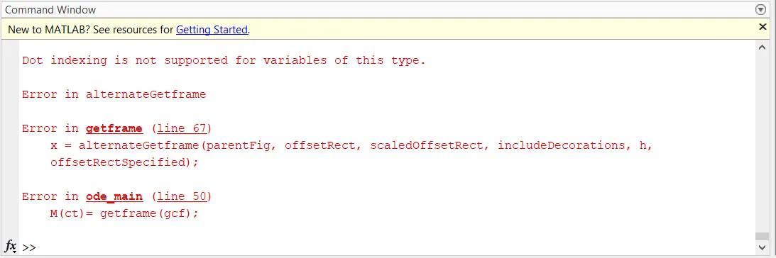
Errors were faced during creating animation video from getframe command. Later it rectified by making some changes in the syntax.
YOUTUBE LINK OF THE ANIMATING VIDEO
RESULTS AND CONCLUSION
Thus the simulation of Pendulum motion is done in MATLAB by solving ODE using ode45 inbuilt. And have gained knowledge on ode45 by browsing and have experienced in creating animation in MATLAB.