Week 3 - Solving second order ODEs

PROGRAM TO SOLVE AN ODE EQUATION AND ANIMATE THE SIMPLE PENDULUM

AIM :

The objective of this challange is to solve the 2nd order ODE equation into 1st order equation and then animate the motion of a oscillating simple pendulum which is the output of the equation derived.

ODE DESCRIPTION :

The ODE is defined as ordinary differential equation, in mathematics an ODE is a differential equation containing one or more functions of one independent variable and the derivatives of those functions.

The ODE which we are dealing with in this is a ODE of motion of a simple pendulum as follows :

here b = damping coefficient = 0.05

m = mass = 1 kg

g = acceleration due to gravity = 9.81 m/s^2

L = length of spring = 1 metre(m)

SIMPLE PENDULUM MOTION :

Basically simple pendulum is a oscillating to and fro motion mechanism which is used widley in our daily lifes

• Used in the wall clocks for Time purposes.
• Used in the sensing of earth quakes and adjust the grounds which is known as friction pendulums.
• Used in keeping the music beats.
• Used in the circus feats for magicians.

EQUATION REDUCTION :

Firstly this given 2nd order equation will be reduced to 1st order equation i.e., ordinary differential equation as follows :

equation is : d^2(theta)/dt^2+(b/m)*d(theta)/dt+(g/L)*sin(theta)

substituting......theta = theta1

dtheta/dt = theta2

The final equation will be

d/dt(theta2)+b/m(theta2)+(g/L)sin(theta1) = 0

here d(theta1)/dt = theta2

d(theta2)/dt = -(b/m)theta2-(g/L)sin(theta1)

PROGRAM CODE :

clear all
close all
clc

%initial values
b = 0.05; % damping coefficient
g = 9.81; %accleration due to gravity m/s^2
l = 1; %length of suspended string or bar in meter(m)
m = 1; %mass of the bob at other end in kg

%initial conditions

theta_variation = [0;3]; %angular displacement and angular velocity varies with theta

%time

t_span = linspace(0,20,100); %this is the time upto which pendulum oscillates

%ODE solving

[t,results] = ode45(@(t,theta) ode_function(t,theta,b,g,l,m),t_span,theta_variation);

figure(1)
plot(t,results(:,1)) %this gives the angular displacement values
hold on
plot(t,results(:,2)) %this gives the angular velocity results
hold off
xlabel('time in sec')
ylabel('angular velocity(radians/sec) and displacement(radians)')

ct = 1;
for j = 1:length(t_span)
x1 = l*sin(results(j,1)); %here (j,1) denotes for each value of j and 1 is angular displacement
y1 = l*cos(results(j,1));

plot([-1 1],[0 0],'linewidth',6,'color','b') %plot for the supporting bar for pendulum
hold on
plot([0 x1],[0 -y1],'linewidth',3,'color','k'); %plot for the string of the pendulum
plot(x1,-y1,'.','markersize',80,'color','r'); %plot for the bob that can be created by the marker command
axis([-4 4 -2.5 0.5])
pause(0.2) %this denotes time between each frame in the movie

M(ct) = getframe(gcf);
hold off 
ct = ct+1;

end

%making a movie of a simple pendulum by attaching all the plots together
movie(M)
videofile = VideoWriter('pendulum_main_sample.avi','Uncompressed avi');
open(videofile)
writeVideo(videofile,M)
close(videofile)

CODE EXPLAINATION :

As we know that we start every code in the editor window with clear all, close all, clc and then code part can be started.

Then initial values like damping coefficient, acceleration due to gravity, length of the string, mass of the body will be given.Then the time span of the motion of the pendulum should be given from 1 to 20 sec and the intervals in between the time period can be given using the command linspace.

Then to solve the ODE equation an inbuilt command called ode45 function is used to solve the ordinary differential equation(ODE) from the data i.e, substitution values which is given earlier in the description below ODE description.

The ode45 function code which is used in the main simple pendulum program is shown below :

function[dtheta_dt] = ode_function(t,theta,b,g,l,m)
theta1 = theta(1);
theta2 = theta(2);
dtheta1_dt = theta2;
dtheta2_dt = -(b/m)*theta2-(g/l)*sin(theta1);
dtheta_dt = [dtheta1_dt;dtheta2_dt];
end

The above ode45 function is executed using the same initially substituted values earlier.

CODE OUTPUT :

The normal curve of the motion of simple pendulum can be visualised by the graph with time on x-axis and angular velocity, displacement on y-axis. This graph variation can be seen by giving different values for damping coefficient, mass of body, length of string. But varyiing the damping coefficient can vary the angular displacement and velocity have a drastic change because if more damping is present more will be friction and viceversa.

The graph for the above ODE equation is shown as below :

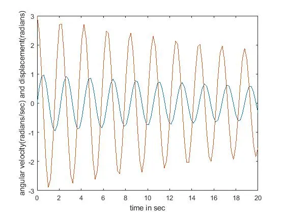
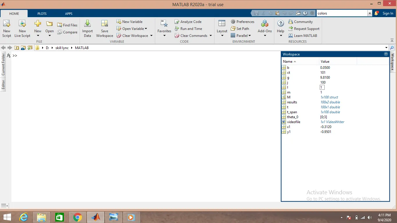
The right side image shows that work space window which contains all the input and output results of ODE equation and input values for geometricality of pendulum.

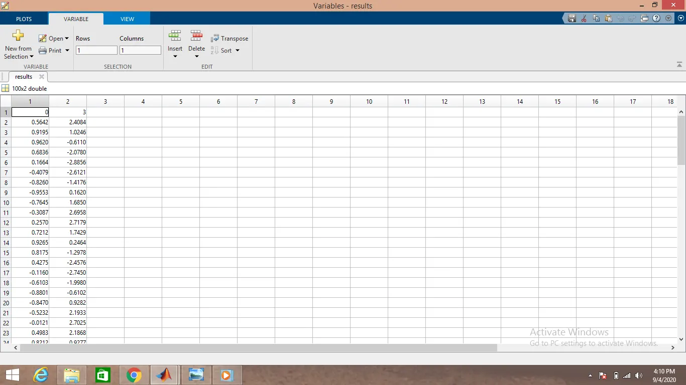
The last image shows the results of the equation which has angular displacement values showing in left column starting with 0 and the angular velocity in the right column which starts from 3. The value will be upto 100 values as number divisions given is 100 in time 1 to 20 seconds.

ERRORS OCCURED:

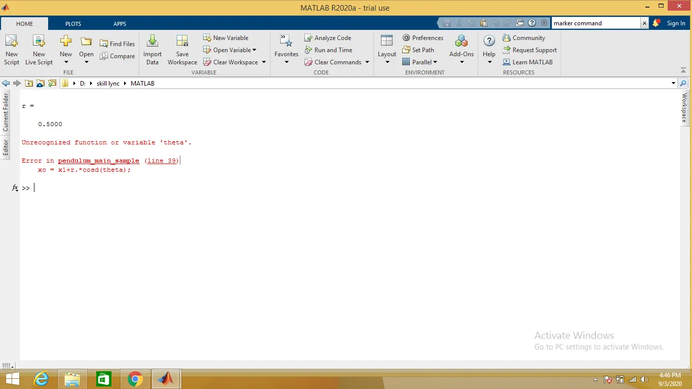
• The error occured at creating bob as when giving a wrong approah to create bob and rectified by using markersize command instead of theta for creating bob.
• The error occured at starting of the loop as instead of giving 1:length(t_span) it was given as 1:length(theta_0) and it was rectified.
• The error which is fixed at the ending of the loop as giving hold off at before ct increment after getframe(gcf) command as that traces the line and same is dispalyed .
• The error occured at giving the axis values for better representation of simple pendulum motion at a perfect position.

CONCLUSION :

The results of the equation can always be changed with a different time period values and the damping coefficient values as this have a important part in the results.

LINK FOR ABOVE PROGRAM :

simple pendulum main program

ODE function code

Youtube link for simple pendulum motion