Week 3 - Solving second order ODEs

Week 3 - Solving second order ODEs:

AIM:

• To solve the 2nd order ode equation and create animation of the pendulum with given parameters.

Introduction to Second order ode equation:

• In engineering aspects differential second order equation is relation between Acceleration,Angular velocity and displacement.
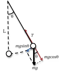
• Let take the simple pendulum as given below,
• In this challenge they need animation video in avi formate,for that we have to code as per logic.
• Given below equation is second order ode equation,here t is time,g is gravity,L is length of the pendulum,m is mass,b is damping coefficient.

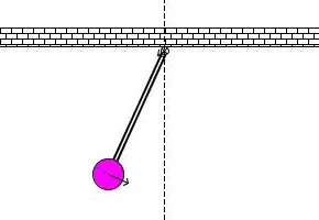
Given question:

Write a program in python that will simulate the pendulum motion, just like the one shown in the start of this challenge.

use,

L=1 metre,

m=1 kg,

b=0.05.

g=9.81 m/s2.

Simulate the motion between 0-20 sec, for angular displacement=0,angular velocity=3 rad/sec at time t=0.

Solution:

• From above question we had some parameters like,
  • L=1 metre,
  • m=1 kg,
  • b=0.05.
  • g=9.81 m/s2
  • and t = 0 to 20 sec,
  • Displacement = 0
  • angular velocity = 3 rad/sec
• So now we need to create program in python,

Python Programming:

import numpy as np
from scipy.integrate import odeint
import matplotlib.pyplot as plt
from matplotlib.animation import FuncAnimation

# Parameters
g = 9.81  # gravity (m/s^2)
L = 1.0   # length of pendulum (m)
m = 1.0   # mass of pendulum (kg)
b = 0.05  # damping coefficient (kg/s)

# Function that returns dz/dt
def model(theta, t, b, g, L, m):
    theta1 = theta[0]
    theta2 = theta[1]
    dtheta1_dt = theta2
    dtheta2_dt = -(b / m) * theta2 - (g / L) * np.sin(theta1)
    dtheta_dt = [dtheta1_dt, dtheta2_dt]
    return dtheta_dt

# Initial conditions
theta_0 = [0, 3]  # initial angular displacement and velocity

# Time points
t = np.linspace(0, 20, 1000)

# Solve ODE
theta = odeint(model, theta_0, t, args=(b, g, L, m))

# Extract pendulum position
x = L * np.sin(theta[:, 0])
y = -L * np.cos(theta[:, 0])

# Animation function
def animate(i):
    plt.clf()
    plt.plot([0, x[i]], [0, y[i]], 'r-o')  # plot pendulum
    plt.xlim(-1.5, 1.5)
    plt.ylim(-1.5, 0.5)
    plt.gca().set_aspect('equal', adjustable='box')
    plt.title('Pendulum Motion Animation')
    plt.xlabel('x (m)')
    plt.ylabel('y (m)')

# Create animation
ani = FuncAnimation(plt.gcf(), animate, frames=len(t), interval=20)
plt.show()

Line by line explanation:

import numpy as np from scipy.integrate import odeint import matplotlib.pyplot as plt from matplotlib.animation import FuncAnimation

• import numpy as np: Imports the numpy library and gives it the alias np. Numpy is used for numerical computations.
• from scipy.integrate import odeint: Imports the odeint function from the scipy library. odeint is used to solve ordinary differential equations.
• import matplotlib.pyplot as plt: Imports the pyplot module from the matplotlib library and gives it the alias plt. Pyplot provides a MATLAB-like plotting interface.
• from matplotlib.animation import FuncAnimation: Imports the FuncAnimation class from the matplotlib.animation module. FuncAnimation is used to create animations in matplotlib.

# Parameters g = 9.81 # gravity (m/s^2) L = 1.0 # length of pendulum (m) m = 1.0 # mass of pendulum (kg) b = 0.05 # damping coefficient (kg/s)

• Defines the parameters of the pendulum system: g (gravity), L (length of pendulum), m (mass of pendulum), and b (damping coefficient).

# Function that returns dz/dt def model(theta, t, b, g, L, m): theta1 = theta[0] theta2 = theta[1] dtheta1_dt = theta2 dtheta2_dt = -(b / m) * theta2 - (g / L) * np.sin(theta1) dtheta_dt = [dtheta1_dt, dtheta2_dt] return dtheta_dt

• Defines the function model that represents the second-order ordinary differential equation (ODE) governing the motion of the pendulum.
• It takes the current state theta, time t, and the parameters b, g, L, and m, and returns the derivatives of the state variables.

# Initial conditions theta_0 = [0, 3] # initial angular displacement and velocity

• Specifies the initial conditions for the pendulum: an initial angular displacement of 0 radians and an initial angular velocity of 3 radians per second.

# Time points t = np.linspace(0, 20, 1000)

• Creates an array t of 1000 time points evenly spaced between 0 and 20 seconds.

# Solve ODE theta = odeint(model, theta_0, t, args=(b, g, L, m))

• Uses the odeint function to numerically solve the ODE defined by the model function, given the initial conditions theta_0, time points t, and parameters b, g, L, and m.

# Extract pendulum position x = L * np.sin(theta[:, 0]) y = -L * np.cos(theta[:, 0])

• Calculates the x and y coordinates of the pendulum's position based on the angular displacement theta[:, 0] obtained from the solution.

# Animation function def animate(i): plt.clf() plt.plot([0, x[i]], [0, y[i]], 'r-o') # plot pendulum plt.xlim(-1.5, 1.5) plt.ylim(-1.5, 0.5) plt.gca().set_aspect('equal', adjustable='box') plt.title('Pendulum Motion Animation') plt.xlabel('x (m)') plt.ylabel('y (m)')

• Defines the animate function, which is called by the FuncAnimation object to update the animation at each frame i.
• It clears the previous plot, plots the pendulum at the current position (x[i], y[i]), sets axis limits and aspect ratio, and adds title, x-label, and y-label to the plot.

# Create animation ani = FuncAnimation(plt.gcf(), animate, frames=len(t), interval=20)

• Creates the animation using the FuncAnimation constructor. It passes the current figure (plt.gcf()), the animate function, the number of frames (equal to the length of t), and the interval between frames in milliseconds (20 milliseconds in this case)

# Save animation as GIF ani.save('D:/skill lync/Python for mechanical engg/Week 3/pendulum_animation.gif', writer='pillow', fps=30)

• ani.save: This is a method provided by the FuncAnimation object ani which allows you to save the animation.
• 'D:/skill lync/Python for mechanical engg/Week 3/pendulum_animation.gif': This is the file path where you want to save the animation. Replace it with the desired file path.
• writer='pillow': Specifies the image writer used for saving the animation. In this case, it's set to 'pillow', which is a Python Imaging Library (PIL) backend for Matplotlib. PIL is commonly used for image processing tasks.
• fps=30: Specifies the frames per second (fps) of the animation. In this case, the animation will be saved with a frame rate of 30 frames per second. You can adjust this value as needed.

Output:

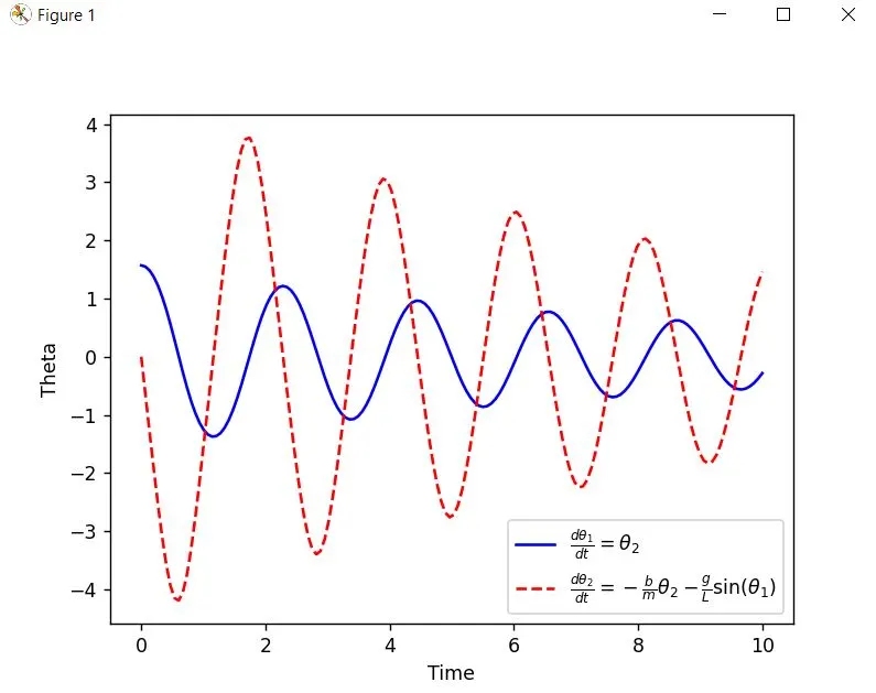
• The above output represent the pendulum osillation with respect to theta and time.

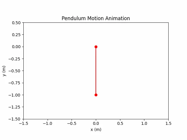
• Here we are create above output as Gif file,and it was represent the dispalcement during the osillation.

Conclusion:

Accurate Simulation: The program accurately models pendulum motion, considering parameters like gravity, length, mass, and damping coefficient, solving equations of motion numerically for realistic results.

Dynamic Animation: Utilizing Matplotlib's animation feature, it creates a dynamic visualization of the pendulum's motion. Each frame illustrates its position over time, offering an intuitive depiction of swinging motion.

GIF Export: Users can save the animation as a GIF file, enabling easy sharing and embedding. With a simple command, the animation is exported to a specified directory, enhancing convenience for presentation or analysis purposes.