Week 3 - Solving second order ODEs
simple pendulum - ODE
Procedure
- the requierd modules are imported
- funtion is defined and the equation to solve is provided
- inputs given and initial condition provided
- time input provided
- result ploted
Program
import numpy as np
from scipy.integrate import odeint
import math
import matplotlib.pyplot as plt

 #defining function
def model(theta,t,b,g,l,m):
	theta1 = theta[0]
	theta2 = theta[1]
	dtheta1_dt = theta2
	dtheta2_dt = (-b/m)*theta2 - (g/l)*math.sin(theta1)
	dtheta_dt = [dtheta1_dt,dtheta2_dt]
	return dtheta_dt

#inputs
b = 0.05
g = 9.81
l = 1
m  = 1

#initial condition
theta_0 = [0,3]
#time point
t = np.linspace(0,10,150)
#solve ODE
theta =odeint(model,theta_0,t,args=(b,g,l,m))

#plot
plt.plot(t,theta[:,0],'b-')
plt.plot(t,theta[:,1],'r--')
plt.xlabel('time')
plt.ylabel('plot')
plt.show()


#oscilation
#Base points for pendulum
x0 = 0
y0 = 0

ct = 0

#Pendulum animation
angles = theta[:,0]
for point in angles:
	filename = str(ct) + '.png' #
	ct = ct+1
	plt.figure()
	x1 = l*math.sin(point)
	y1 = -l*math.cos(point)
	plt.xlim([-1.5,1.5])
	plt.ylim([-1.5,0.1])
	plt.plot(x0,y0,marker='o')
	plt.plot(x1,y1,marker = 'o', ms = 10)
	plt.plot([x0,x1],[y0,y1])
	plt.savefig(filename)
Result
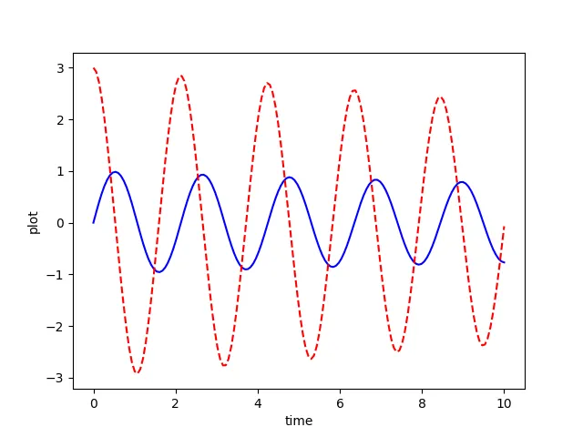
Here the red doted line shows displacement and blue line shows angular velocity
Animation