Week 3 - Solving second order ODEs

objective

write a program that solves the following ODE. This ODE represents the equation of motion of a simple pendulum with damping

using pythone ode function can also be solve which can be seen in up coming simple pemdulum proble solution

solution procedure using ode function first order ode can be solved but simple pensulun is a second order ode proble to ove come that proble theta1 and theta2 defined using these ode function are solved

program

##simple pensdulum
import numpy as np
from scipy.integrate import odeint
import matplotlib.pyplot as plt 
import math 


#function defination
def model(theta,t,b,g,l,m):
    theta1=theta[0];
    theta2=theta[1];
    dtheta1_dt=theta2;
    dtheta2_dt=-(b/m)*theta2-(g/l)*math.sin(theta1);
    dtheta_dt=[dtheta1_dt,dtheta2_dt];
    return dtheta_dt;

#input paramtes
b=0.15;#damping coeffiecint
g=9.81;#in m/s^2
l=1;#length of wire/rope in m
m=1;#mass in kg

#intial condotion
theta_0=[math.pi/2,0];

#time points
t=np.linspace(0,20,150);

#solve ode
theta=odeint(model,theta_0,t,args=(b,g,l,m))#ode solver

#plot results
plt.figure(1)
plt.plot(t,theta[:,0],'b-',label=r'$\frac{d\theta_1}{dt}=theta2$');
plt.plot(t,theta[:,1],'r--',label=r'$\frac{d\theta2}{dt}=-\frac{b}{m}\theta2-\frac{g}{l}sin\theta_1$')
plt.xlabel('time')
plt.ylabel('plot')
plt.legend(loc='best')
ct=2
#animation
for x in theta[:,0]:
    x0=0;
    y0=0;
    x1=l*math.sin(x)
    y1=-l*math.cos(x);
    fl=str(ct)+'.png'
    ct=ct+1
    
    fig=plt.figure(ct)
    plt.plot([x0,x1],[y0,y1])
    plt.plot(x1,y1,'-o')
    plt.xlim([-2,2])
    plt.ylim([-2,2])
    plt.savefig(fl)
    

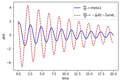
time vs displacement and velocity plot

animation zip file of pendulum

https://drive.google.com/file/d/1_A4IDYMM4OpYS9z67nL-JiazpeNISOx1/view?usp=sharing