Week 3 - Solving second order ODEs

AIM : To write a program to simulate the transient behaviour of a simple pendulum and to create an animation of it's motion.

PROBLEM STATEMENT:

An ODE is used to describe the transient behavior of a system. In mechanics and physics, the simple harmonic motion is a special type of periodic motion where the restoring force on the moving object is directly proportional to, and opposite of, the object's displacement vector.

In real time scenarios the air resistance slows down the velocity of the simple pendulum and for the same reason damping factor is introduced in the equation given below. Hence it is called as damped simple harmonic motion. (the oscillations are damped). From Newton's second law, an ODE is obtained for the motion of simple pendulum as shown in the figure below. The angular displacement and angular velocity are represented in the equation.

EQUATION USED :

`(d^2 theta)/(dt^2) + b/m*(d(theta))/dt+g/Lsintheta = 0`

In the above equation :

• g = gravity in m/s2,
• L = length of the pendulum in m,
• m = mass of the ball in kg,
• b=damping coefficient.
• `theta` = angular displacement

INITIAL CONDITIONS :

• L=1 metre,
• m=1 kg,
• b=0.05.
• g=9.81 m/s2.

PYTHON CODE FOR SIMPLE PENDULUM :

# Second order ode
import numpy as np
from scipy.integrate import odeint
import matplotlib.pyplot as plt
import math

# function that returns dz/dt
def model(theta,t,b,g,l,m):

    theta1 = theta[0]
    theta2 = theta[1]
    dtheta1_dt = theta2
    dtheta2_dt = -(b/m)*theta2 - (g/l)*math.sin(theta1)
    dtheta_dt = [dtheta1_dt, dtheta2_dt]
    return dtheta_dt

b = 0.05
g = 9.81
l = 1
m = 1

# Initial condition 
theta_0 = [0,3]

# time points
t = np.linspace(0,20,200)

# Solve ODE
theta = odeint(model,theta_0,t,args = (b,g,l,m))

#plot results
plt.plot(t,theta[:,0],'b-',label=r'$\frac{d\theta_1}{dt}=\theta2$')
plt.plot(t,theta[:,1],'r--',label=r'$\frac{d\theta2}{dt}=-\frac{b}{m}\theta_2-\frac{g}{L}sin\theta_1$')
plt.ylabel('plot')
plt.xlabel('time')
plt.legend('best')
plt.savefig('output.png')
plt.show()

# To creat animation
ct = 1
x0 = 0
y0 = 0

for i in theta[:,0]:
    x1 = x0 + (l*math.sin(i))
    y1 = y0 + (-l*math.cos(i))

    filename = str(ct) + '.png'
    ct = ct + 1

    plt.figure()
    plt.plot([-1,1],[0,0],"black")
    plt.plot([x0,x1],[y0,y1],"red")
    plt.plot(x1,y1,'o',markersize = '20')
    plt.xlim([-1.5,1.5])
    plt.ylim([-1.5,1.0])
    plt.savefig(filename)

EXPLANATION OF CODE :

• At first math, matplotlib, numpy and scipy modules were imported for their various functions.
• Initial inputs such as b,g,l,m are provided according to data in the question.
• An array of initial theta was created to define initial angular displacement and initial angular velocity.
• An array of time span was created to store 200 equally spaced intervals between time 0 to 20 seconds.
• To solve the second order ODE, a function named ode_function which stores the above matrix data in it.
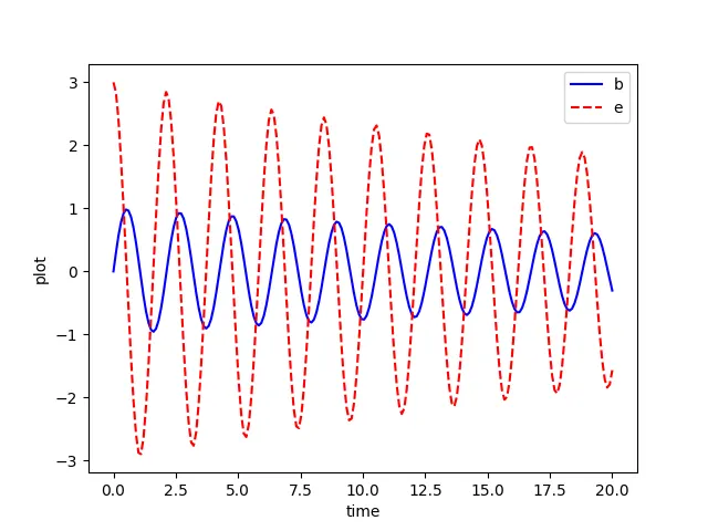
• The given second order ODE was solved using 'odeint' command followed by proper syntax of the calling function and the result obtained was used to plot the graph of variation of angular displacement and angular velocity wrt time.
• Now for creating the animation of obtained harmonic motion of pendulum, for loop was used and a loop counter variables was initiated,the values of angular position is stored in a separate variable called 'tmp' and is iterated in for loop.
• In this execution the one end of the string of pendulum was fixed and the other end moves according to the solution of the ODE solved and was plotted for each time interval of the time span.

OUTPUT :

RESULT :

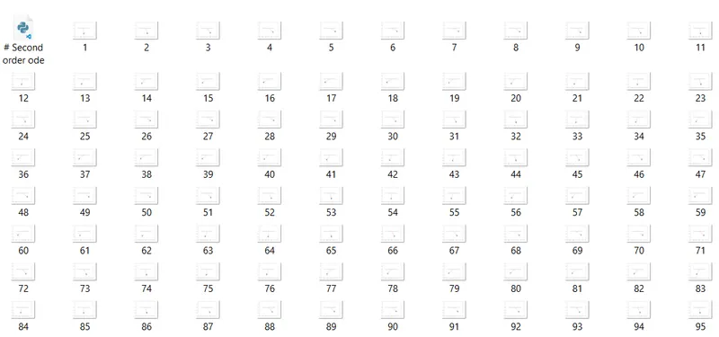
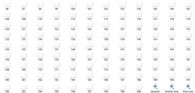
• All the images are saved in the folder and we have to conver those images into the gif.
• We get 200 images and therefore we have convert those images into gif by using imagemagick.

ANIMATION VIDEO LINK :

https://drive.google.com/file/d/1i4grkvoDhWeL8x5YvVTd4OKo0ZW1V2vz/view?usp=share_link

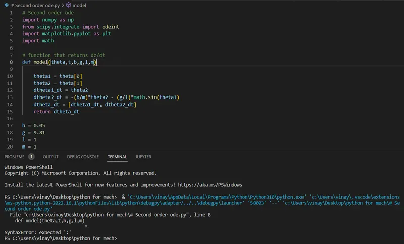
ERRORS OCCERED :

SOLUTION :

• It is a syntax error. We have to keep the semicolon ':' at the end of the function line.
• The spelling of the names should be exact as we given before in the same programme.
• We have to give the initial conditions for every term.
• The libraries should be import according to the problems we are solving.

CONCLUSION :

• The above graph shows the angular displacement and angular velocity and it changes over the time due to the effect of the damping, the values of reduce angular displacement and angular velocity with time as is clearly visible in above plot.