Week 3 - Solving second order ODEs

Aim:

The project aims to stimulate the movement of the simple pendulum(0-20s) which moves according to the below second order differential equation(ODE) and to create an animation of its movement using Python.

 d2θdt2+bm⋅(dθdt)+gl(sin⁡θ)=0">d^2θ/dt^2+b/m(dθ/dt)+g/l(sinθ)=0

where:

b - damping coefficient

l - Length of the string

g - acceleration due to gravity

m - the mass of the bob

Procedure: 

The equation of simple pendulum using damping is a second-order differential equation(ODE). So, it  must be divided into  two lower-order differential equations as

dθ1dt=θ2">dθ1/dt=θ2

dθ1dt=θ2">dθ1/dt=θ2

dθ2dt=-(bm)⋅θ2-(gl)⋅sinθ1">dθ2/dt=−(b/m)⋅θ2−(g/l)⋅sinθ1

However, some assumptions are made for converting the second order ode to first order ode.

they are 

θ=θ1">θ=θ1

dθdt=dθ1dt=θ2">dθ/dt=dθ1/dt=θ2

d2θdt2=ddt(dθ1dt)=dθ2dt">d^2θ/dt^2=d(dθ1/dt)dt=dθ2/dt

Code:

• Import numpy, matplotlib, math modules for array, plotting and math operations respectively.
• The \'odeint\' module extracted from \'scipy.integrate\' module to solve the given ode.
• Divide higher-order ODE into the first-order ODE and define in the function.
• Define the initial conditions and angular velocity and displacement. The simulation time is taken in the range of 0-20 seconds.
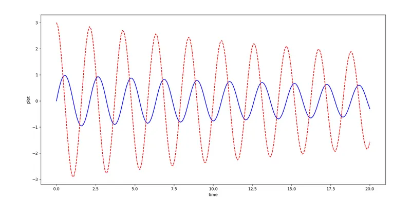
• To solve the ODE call the odeint module and given the define variables. Then plot graph between the time vs displacement and time vs angular velocity.

import math
import numpy as np
import matplotlib.pyplot as plt
#from matplotlib import animation
#from matplotlib.animation import pillowriter
from scipy.integrate import odeint

def model(theta,t,b,g,l,m):

    theta1 = theta[0]
    theta2 = theta[1]
    dtheta1_dt = theta2
    dtheta2_dt = -(b/m)*theta2 -(g/l)*math.sin(theta1)
    dtheta_dt = [dtheta1_dt, dtheta2_dt]
    return dtheta_dt

b = 0.05
g = 9.81
l =1
m =1

#initial condition
theta_0 = [0,3]

#time points
t = np.linspace(0,20,200)


 #solve ODE
theta = odeint(model,theta_0,t,args=(b,g,l,m))



#plot results
plt.figure(1)
plt.plot(t,theta[:,0],'b-',label =r'$\frac{d\theta_1}{dt} = \theta2$')
plt.plot(t,theta[:,1],'r--',label =r'$\frac{d\theta_2}{dt} =-\frac{b}{m}\theta2-\frac{g}{L}sin\theta_1$')
line = plt.plot([0,0],[3,3])
plt.plot(l,m,'-', linewidth = 3,color = 'b')
plt.ylabel('plot')
plt.xlabel('time')
plt.show()

ct =1
theta_1 = theta[:,0]
for t in theta_1:
    x0 = 0
    y0 =0
    x1 = l*math.sin(t)
    y1 = -l*math.cos(t)

    filename= str(ct) +'.png'
    ct= ct + 1

    #plotting
    plt.figure()
    plt.plot([-0.5,0.5],[0,0],color ='black',linewidth = 3)
    plt.plot([x0,x1],[y0,y1],color = 'r',linewidth = 3)
    #plt.plot(x0,y0,'o',markersize = 5)
    plt.plot(x1, y1, 'o', markersize=30, color='blue')
    plt.xlim([-1.5, 1.5])  # defining the x limit.
    plt.ylim([-1.5, 1.5])  # defining the y limit.
    plt.title('Animation of of Simple Pendulum')
    plt.savefig(filename)