Project 2 - Rankine cycle Simulator

clear all 
close all
clc

T1 = input('enter the temperature at inlet of the turbine(in degree c) =');
P1 = input('enter the pressure at inlet of the turbine(in bar) =' );
P2 = input('enter the pressure at inlet of the condenser(in bar) =');

t = linspace(0,373.15,200);
disp('')

% calculating and displaying the values of P,T,h,s for each state using

%at state point 1

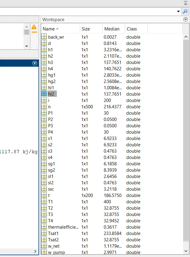
h1 = XSteam('h_pT',P1,T1);
s1 = XSteam('s_pT',P1,T1);
hl1 = XSteam('hL_p',P1);
hg1 = XSteam('hv_p',P1);
sl1 = XSteam('sL_p',P1);
sg1 = XSteam('sV_p',P1);
Tsat1 = XSteam('Tsat_p',P1);

% at state point 2

s2 = s1;
sl2 = XSteam('sL_p',P2);
sg2 = XSteam('sV_p',P2);
d = (s2 - sl2)/(sg2-sl2);
hl2 = XSteam('hL_p',P2);
hg2 = XSteam('hV_p',P2);
h2 = hl2 + d*(hg2-hl2);
T2 = XSteam('T_ph',P2,h2);
Tsat2 = XSteam('Tsat_p',P2);

% at state 3

h3 = hl2;
s3 = sl2;
P3 = P2;
T3 = T2;

% at state 4

s4 = s3;
P4 = P1;
h4 = XSteam('h_ps',P4,s4);
T4 = XSteam('T_ps',P4,s4);

% work and efficiency calculations

% work done by the turbine
w_turbine = h1-h2;
% work done by pump
w_pump = h4-h3;

% net work done 

w_net = w_turbine - w_pump;

thermalefficiency = (1 - (h2 - h3)/(h1-h4));
back_wr = w_pump/w_turbine;

ssc = 3600/w_turbine;

% plottingT-s curves

figure(1),clf
hold on

for i=1:length(t)
    plot(XSteam('sL_T',t(i)),t(i),'g')
    plot(XSteam('sV_T',t(i)),t(i),'g')
end

%cycle

plot([s1 s2],[T1 T2],'LineWidth',2)
text(s1,T1,'1','FontSize',15)
if d>1
    T3 = Tsat2;
    plot([s2 sg2 s3 s4],[T2 Tsat2 T3 T4],'LineWidth',2)
    T2 = Tsat2;
    text(s2,T2,'2','FontSize',15)
    text(s3,T3,'3','FontSize',15)
else
    plot([s2 s3 s4],[T2 T3 T4],'LineWidth',2)
    text(s2,T2,'2','FontSize',15)
    text(s3,T3,'3','FontSize',15)
end
n = linspace(T1,T2,500);
for i = 1:length(n)
    plot(XSteam('s_pT',P1,n(i)),n(i),'.','LineWidth',2)
end

plot([sl1 sg1],[Tsat1 Tsat1],'LineWidth',2)
text(sl1,Tsat1,'4','FontSize',15)
xlabel('ENTROPY(KJ/KG-K)')
ylabel('TEMPERATURE(K)')
title('T-s graph')

%h-s graph
figure(2),clf
hold on

% saturation curve

for i=1:length(t)
    plot(XSteam('sL_T',t(i)),XSteam('hL_T',t(i)),'r.')
    plot(XSteam('sV_T',t(i)),XSteam('hV_T',t(i)),'r.')
end

%cycle

plot([s1 s2 s3 s4 s1],[h1 h2 h3 h4 h1],'LineWidth',2)
text(s1,h1,'1','FontSize',15)

text(s2,h2,'2','FontSize',15)
text(s3,h3,'3','FontSize',15)
text(s4,h4+90,'4','FontSize',15)

xlabel('ENTROPY(KJ/KG-K)')
ylabel('TEMPERATURE(K)')
title('h-s graph')

%displaying the results in the command window

%at state point1:

disp('at state point 1:')
fprintf('P1 = %.2f bar n',P1)
fprintf(['T1 = %.2f' char(176) 'c n'],T1)
fprintf('h1 = %.2f KJ/KG n',h1)
fprintf('s1 = %.2f KJ/KGK n',s1)
disp(' ')


%at state point2:

disp('at state point 2:')
fprintf('P2 = %.2f bar n',P2)
fprintf(['T2 = %.2f' char(176) 'c n'],T2)
fprintf('h2 = %.2f KJ/KG n',h2)
fprintf('s2 = %.2f KJ/KGK n',s2)
disp(' ')

%at state point3:

disp('at state point :')
fprintf('P3 = %.2f bar n',P3)
fprintf(['T3 = %.2f' char(176) 'c n'],T3)
fprintf('h3 = %.2f KJ/KG n',h3)
fprintf('s3 = %.2f KJ/KGK n',s3)
disp(' ')


%at state point4:

disp('at state point 4:')
fprintf('P4 = %.2f bar n',P4)
fprintf(['T4 = %.2f' char(176) 'c n'],T4)
fprintf('h4 = %.2f KJ/KG n',h4)
fprintf('s4 = %.2f KJ/KGK n',s4)
disp(' ')


fprintf('work done by turbine = %.2f kj/kg n',w_turbine)
fprintf('work done by pump = %.2f kj/kg n',w_pump)
fprintf('net work done = %.2f kj/kg n',w_net)
fprintf('thermalefficiency = %.2f %% n',thermalefficiency)
fprintf('Back-work ratio = %f n',back_wr)
fprintf('specific steam conductivity = %.2f kg/kwh n',ssc)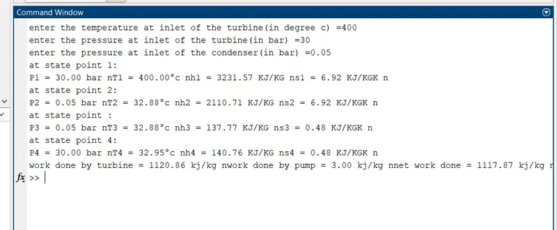

EXPLANATION:

- giving inputs.
- calculating and displaying the values of P,T,h,s for each state using.
- at state point 1
- at state point 2
- at state point 3
- at state point 4
- work and efficiency calculations
- calculating work done by the turbine
- calculating work done by pump
- calculating net work done
- plottingT-s curves
- plottingh-s curves
- displaying the results in the command window at state point 1,2,3,4.
- and writing for output