Week 3 - Solving second order ODEs

Aim: -

Writing a Python program that solves the following ODE. This ODE represents the equation of motion of a simple pendulum with damping.

Objectives: -

1. Able to simulate Pendulum motion.
2. Able to plot Displacement vs time graph.

Description: -

The way the pendulum moves depends on Newton's second law of motion. When this law is written down, we get a second order Ordinary Differential Equation that describes the position of the "ball" w.r.t time & describes the transient behavior of a system.

The ode of the pendulum is described below

d2θdt2+bm⋅dθdt+gL⋅sinθ=0d2θdt2+bm⋅dθdt+gL⋅sinθ=0

assume

θ=θ1θ=θ1

dθdt=dθ1dt=θ2dθdt=dθ1dt=θ2

d2θdt2=ddt(dθ1dt)=ddt(θ2)d2θdt2=ddt(dθ1dt)=ddt(θ2)

dθ2dt=−bmθ2−glsinθdθ2dt=-bmθ2-glsinθ

In the above equation,

• gravity g = 9.81 m/s2,
• length of the pendulum L = 1 m,
• mass of the ball m = 0.1 kg,
• damping coefficient b=0.05
• time interval = 0-20sec
• for angular displacement=0, angular velocity=3 rad/sec at time t=0 sec.

Procedure: -

1. Create an model function program for second order Ordinary Differential Equation of pendulum with dtheta_dt as function output & t,theta,b,g,l,m as input variables.
2. Give values to input variables.
3. Solve ode for given inputs.
4. plot a graph between angular displacement, angular velocity vs time interval.
5. creating for loop to trace the movement of the pendulum.
6. create a horizontal reference line and vertical string line one end of the string line is fixed and another end depends on sine and cosine angles.
7. Plot the bob with a marker at the end of the string.
8. Define axis range, the grid on.
9. Save each frame and increment the loop by one.
10. use image magick to stitch the frames to form a .gif file

Main Program: -

# 2nd order ODE


import math                         # importing math library
import matplotlib.pyplot as plt     # importing ploting library  
from scipy.integrate import odeint  # importing Scipy.integrate package using function ODEINT
import numpy as np                  # importing numpy module

# ODE function that returns dz/dt
def model(theta,t,b,g,L,m):        
	theta1 = theta[0]
	theta2 = theta[1]
	dtheta1_dt = theta2
	dtheta2_dt = -(b/m)*theta2-(g/L)*math.sin(theta1)
	dtheta_dt = [dtheta1_dt, dtheta2_dt]
	return dtheta_dt

# inputs
b = 0.05   #damping coefficient
g = 9.81   #gravity in m/s2
L = 1      #length of the pendulum in m
m = 1      #mass of the ball in kg

# initial condition at t = 0 sec displacement=0, angular velocity=3 rad/sec
theta_0 = [0, 3]

# time points
t = np.linspace(0,20,400)

# solve ODE
#from scipy.integrate import odeint

results = odeint(model,theta_0,t, args = (b,g,L,m))

# plot results 
plt.figure(1)
plt.plot(t,results[:,0],'b-',label = r'$\frac{d\theta1}{dt}=\theta2$')
plt.plot(t,results[:,1],'r--',label = r'$\frac{d\theta2}{dt}=- \frac{b}{m}\theta2-\frac{g}{L}sin\theta_1$')
plt.xlabel('Time interval');
plt.ylabel('angular velocity-acclelaration');
plt.legend(loc = 'best')
plt.grid('on')
plt.show()

#print(results)

ct = 1
n = 300
for i in np.linspace(0,n,n+1):
	#print(i)
	#print(results[i,0])
	i = int(i)
	if i < n:
		#print(i)
		# fixed and swing handing position
		x0 = 0
		y0 = 0
		# end position of string and bob center position
		x1 =  L * math.sin(results[i,0])
		y1 = -L * math.cos(results[i,0])

		figure = str(ct) + '.png'
		ct = ct + 1
		# creating positional images of pendulum motion 
		plt.figure()
		plt.plot([-1, 1], [0, 0],color='k',linewidth=3)    # fixed wall
		plt.plot([x0, x1],[y0, y1],color='b',linewidth=3)  # string
		plt.plot(x1, y1, marker='o',markerfacecolor='r', markersize=30)  # bob 
		plt.title('Pendulum motion')
		plt.xlim([-1.25,1.25])
		plt.ylim([-1.25,0.25])
		plt.grid('on')
		plt.savefig(figure)
	
#plt.show()

 

Output/Result graph: -

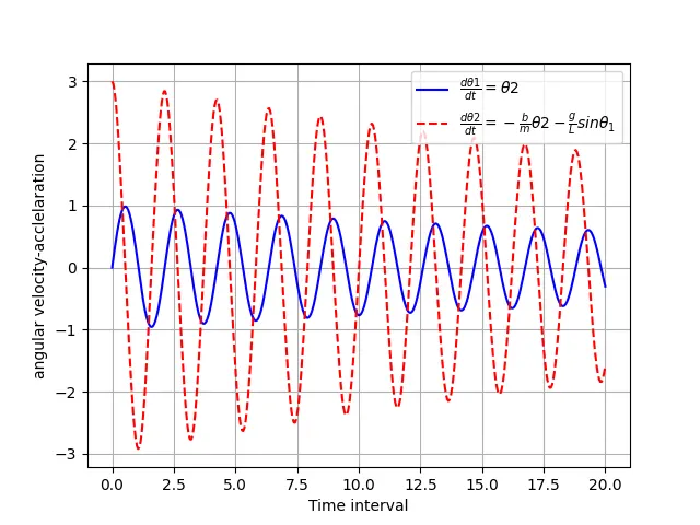
Video is attached below