Week 3 - Solving second order ODEs

1. INTRODUCTION

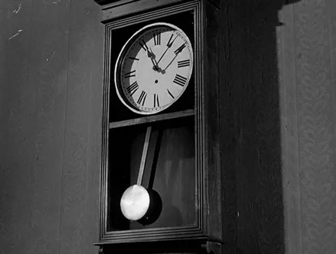
The pendulum is a body or mass suspended from a fixed point so that it can swing back and forth under the influence of gravity. Pendulums are used to regulate the movement of clocks because the interval of time for each complete oscillation, called the period, is constant. The period depends on the length of the pendulum and also to a slight degree on the amplitude, and the width of the pendulum's swing.

2. AIM

To solve the second-order ode function using Matlab which depicts the motion of the pendulum and to create an animation of the same.

3. OBJECTIVE

To write a program that solves the following ODE. This ODE represents the equation of motion of a simple pendulum with damping

In the above equation,

g = gravity in m/s2,

L = length of the pendulum in m,

m = mass of the ball in kg,

b=damping coefficient.

FIXED PARAMETERS

Length (L) =1 metre,

Mass (m) =1 kg,

Damping coiefficient (b) =0.05.

Acceleration due to gravity (g) =9.81 m/s2.

For Time period = 0-20 sec

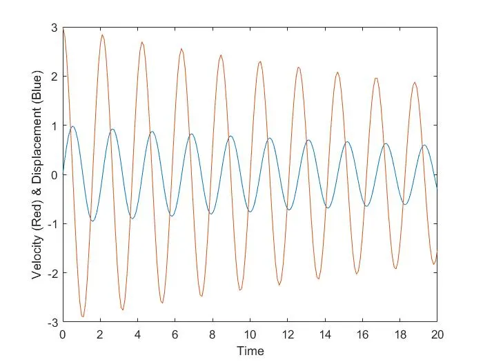
Angular displacement=0, Angular velocity=3 rad/sec at time t=0.

4. FUNCTION CODE

% ODE Function
function dtheta_dt = ode_funs(t,theta,b,g,l,m); 
theta1 = theta(1); 
theta2 = theta(2); 
dtheta1_dt = theta2; 
dtheta2_dt = ‐(b/m)*theta2‐(g/l)*sin(theta1);
dtheta_dt = [ dtheta1_dt ; dtheta2_dt];
end

MAIN PROGRAM:-

clear all
close all
clc

%values
b=0.05; %damping co-efficient
g=9.81; %gravity
m=1; %mass
l=1;

%initial condition
t_span=linspace(0,20,200); %time integrate
theta_0=[0;3]; %angular displacement =0,angular velocity=3.

%solve differential equation
[t,results]=ode45(@(t,theta)ode_func(t,theta,l,g,b,m),t_span,theta_0)

%plot the values
figure(1)
plot(t,results(:,1)) %time vs displacement
hold on
grid on
xlabel('time')
ylabel('angular displacement & angular velocity')
legend('angular displacement & angular velocity')

%animation
ct=1;
for i=1:length(results(:,1))

%initial location
x0=0;
y0=0;

%final location
x1=l*sin(results(i,1));
y1=-1*cos(results(i,1));

figure(2)
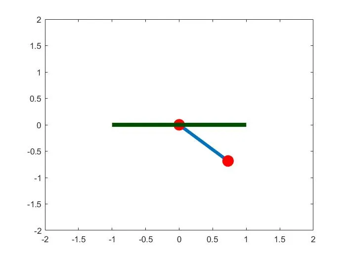
plot([-1 1],[0 0],'linewidth',6,'color','g'); %creating a beam
axis([-2 2 -2 2]); %fixed axis
line([x0 x1],[y0 y1],'linewidth',2,'color','b'); %creating the line from initial value to final value
hold on
plot(x1,y1,'0','markers',20,'markerfacecolor','r'); %create the sphere attached at end of the rope
hold off
pause(0.10)

% for animation
m(ct)=getframe(gcf);
ct=ct+1;

end

movie(m);
videofile=videowriter('simple_pendulum.avi','uncompressed AVI');
open(videofile)
writevideo(videofile,m)
close(videofile)
Function program

function[dtheta_dt]=ode_func(t,theta,b,g,l,m)

theta1=theta(1) %displacement

theta2=theta(2) %velocity

dtheta1_dt=theta2; %angular velocity

dtheta2_dt=-(b/m)*theta2-(g/l)*sin(theta1); %acceleration

dtheta_dt=[dtheta1_dt;dtheta2_dt];

end

EXPLANATION

• In this function program, the second-order ODE is simplified to the first-order ODE by introducing the term theta1 & theta2.
• Then theta1 & theta2 are differentiated and the dtheta_dt gives a column matrix.

• EXPLANATION

  • In the above program, the fixed parameters are length, mass, damping coefficient, and acceleration due to gravity.
  • Time and angle are given as the initial condition.
  • In the span command, 200 values are taken between 0 to 20 times period.
  • Using the ode 45 command ODE function is introduced.
  • Using the plot command velocity and displacement are plotted on the y-axis against time on the x-axis.
  • Using the for loop command the mass at various points and various times are marked in the graph and are plotted.
  • Using the movie command the plot is saved as an uncompressed avi file.

  6. PLOT

  

  

  7. ANIMATION