Challenge

Week 3 - Solving second order ODEs

AAnirban Polle6 Aug 2022

Objective-To simulate the transient behaviour of a simple pendulum and to animate the oscillation using MATLAB.

Theory-A simple pendulum consists of a relatively massive object hung by a string from a fixed support. It typically hangs vertically in its equilibrium position. The massive object is affectionately referred to as the pendulum bob. When the bob is displaced from equilibrium and then released, it begins its back and forth vibration about its fixed equilibrium position. The motion is regular and repeating, an example of periodic motion.

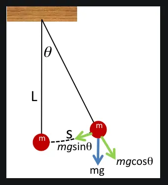
On Solving, We get a Ordinary Differential equation of 2^nd Order that describes the position of the ball with respect to time. The equation is given below:

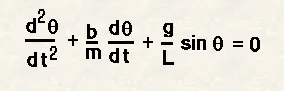
In this Equation:

b= Damping Coefficient, i.e. 0.05

m= mass of the bob i.e. 1 kg

L= Length of the string i.e. 1 m

g= Acceleration due to gravity i.e. 9.8 m/s^2

We need to convert the above given 2^nd order ODE to two 1^st order ODE and simulate the motion.

Code-

% programm simple pendulum

close all

clear all

clc

% ODE simple pendulum inputs

b=0.05; % Damping coefficient

m=1; %mass of bob in kg

g=9.81; % gravity

l=1; % length of string in meter

% Intial conditions

theta_0=[0;3];

% time points

t_span=linspace(0,20,300);

%call the function

[t,results]=ode45(@(t,theta) ode_function(t,theta,b,g,l,m),t_span,theta_0);

%ploting time vs velocity & displacement curve Figure1,

figure(1)

plot(t,results(:,1))

hold on

plot(t,results(:,2))

ylabel('velocity(r) & Displacement(b)')

xlabel('time')

hold off

ct=1;

for i=1:length(t)

x0=0;

y0=0;

x1=l*sin(results(i,1));

y1=-l*cos(results(i,1));

x2=-1;

y2=0;

x3=1;

y3=0;

figure(2)

plot([x0 x1],[y0 y1],'linewidth',3,'color','b')

hold on

plot(x1,y1,'o','markersize',20,'markerfacecolor','r')

plot([x2 x3],[y2 y3],'linewidth',2,'color','g')

axis([-2 2 -2 2]);

pause(0.01);

% Initializing an array to store each frame of graphs

M(ct)=getframe(gcf);

hold off

ct=ct+1;

end

% Generate an Animation

movie(M)

videofile= VideoWriter('Simple pendullum.avi','Uncompressed AVI');

open(videofile)

writeVideo(videofile,M)

close(videofile)

Function code-

% function for simple pendulam

function[dtheta_dt]=ode_function(t,theta,b,g,l,m)

theta1=theta(1);

theta2=theta(2);

dtheta1_dt=theta2;

dtheta2_dt=-(b/m)*theta2-(g/l)*sin(theta1);

dtheta_dt=[dtheta1_dt;dtheta2_dt];

end

Explantion-

Input of value given b,m,L,g.
Create an array theta_0 to store the initial displacement as 0m/s and Initial velocity as 3 rad/sec
Create an array to store time from 0 to 20 with 300 values in between.
Solving the ODE by using function ode45
Defining another function as ode_function to solve the ODE by taking inputs of t, theta, b,g,L,m.
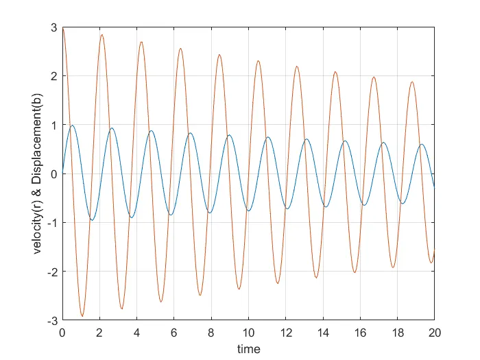
Plot the graph for time vs Displacement and Velocity.
A for loop is used to locate the position of the bob and for each position is stored in array M
Create a movie animation

ERROR-

Forgot hold off command

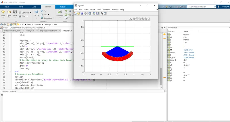
After giving this command it solved.

2.forgot to giving comma character

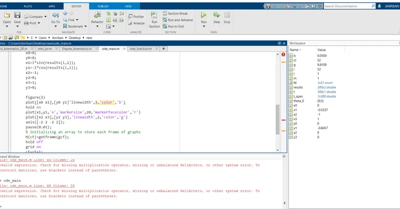
After giving this it solved.

Output-

Plot velocity-displacement and time curve

Animation link-

https://youtu.be/PJeWxUN_zqA

Week 3 - Solving second order ODEs

Ship work like this
in your own course.

Talk to a career counsellor

Ship work like thisin your own course.

Talk to a career counsellor

Ship work like this
in your own course.