Week 3 - Solving second order ODEs

Aim

To solves the ODE which represents the equation of motion of a simple pendulum with damping.

Objective

• To write a program that solves the following ODE which represents the equation of motion of a simple pendulum with damping.

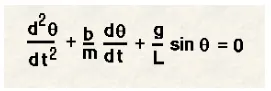
• Write a program that simulate the pendulum motion and create an animated video.

Theory

A simple pendulum consists of a bob suspended at the end of a thread that is so light as to be considered massless. The motion of simple pendulum is periodic motion which is an example of simple harmonic motion. Movement of the pendulum depends on Newton's second law. When this law is written down, a second-order Ordinary Differential Equation is formed that describes the position of the end of the pendulum with respect to time.

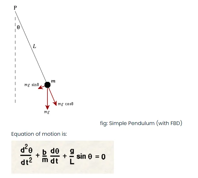
In this equation,

g = Acceleration due to gravity in meter/second^2

L = Length of the pendulum in meter

b = damping constant

m = mass of the bob in kg

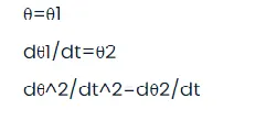
The given equation of motion is in second order, inorder to solve this equation it should be converted into first order

let

Given input,

• L=1 metre
• m=1 kg
• b=0.05
• g=9.81 m/s^2
• Time span= 0-20 sec
• angular displacement=0
• angular velocity=3 rad/sec2 at time t=0

program code

% Programme to create the transient behaviour of pendulum
clear all
close all
clc

b = 0.05;
g = 9.81;
l = 1;
m = 1;

%initial condition
theta_0 = [0;4];

%time plots
t_span = linspace(0,10,500);

%solve ODE
[t,results] = ode45(@(t,theta) ode_func(t,theta, b,g,l,m),t_span,theta_0);

plot(t,results(:,1))
hold on 
plot(t,results(:,2))
xlabel('time')
ylabel('plot')

% Iteration using for loop to create animation of simple pendulum
ct = 1;
theta_1 = results(:,1);
for i = 1:length(theta_1)
    
    % initial co-ordinates
    
    x0 = 0;
    y0 = 0;
    theta_2 = theta_1(i);
    
    % final co-ordinates
    
    x1 = 1*sin(theta_2);
    y1 = -1*cos(theta_2);
    
    % Plotting for animation
    figure(2)
    % Base of the pendulum
    plot([-1,1],[0,0],'linewidth',6,'color','black')
    hold on
    
    % string of the pendulum
    line([x0 x1],[y0 y1],'linewidth',4,'color','b')
    
    % Bob of the pendulum
    plot(x1,y1,'marker','o','markersize',20,'markerfacecolor','magenta')
    axis([-1.5 1.5 -1.5 1])
    pause(0.01)
    hold off
    P(ct) = getframe(gcf)
    ct = ct+1;
end
% Creating movie from gathered frame
   movie(P)
   videofile = VideoWriter('simple_pendulum.avi','Uncompressed AVI');
   open(videofile)
   writeVideo(videofile,P)
   close

Code for function program

function [dtheta_dt] = ode_func(t,theta,b,g,l,m)

theta1 = theta(1)
theta2 = theta(2)
dtheta1_dt = theta2;
dtheta2_dt = -(b/m)*theta2 - (g/l)*sin(theta1);
dtheta_dt = [dtheta1_dt ; dtheta2_dt];
end

Detailed explanation of code

• At first inputs and input conditions are mentioned.
• Time period is given as per the question.
• In order to solve the ODE we use a MATLAB Inbuilt function named as "ode45". The function is used with constant theta, t and another function is used which is defined seperately in function program.
• In function coding, it is named as ode_finc. This is the process of converting second order ODE into first order. the dtheta_dt is a column vector having two column consisting of dtheta1_dt and dtheta2_dt.
• In the next step result of solved ODE is plotted w.r.t time using plot command. Both values of angular displacement and angular velocity are plotted against time.
• xlabel and ylabel commands are used to name the axis.
• For loop is used to create the simulation of pendulum. In the loop the values of theta is stored in 'i'. After that initial conditions are mentiond. x0 and y0 are initial points and it is (0, 0). Theta2 is defined as the value of theta1 when 'i' varies from 1 to length(theta1). Final co-ordinates are found out using trigonometric relations.
• To find the base of the of pendulum plot command is used. A bar is created at linewidth of '4'.
• String of the pendulum is created using the line command by connecting the starting and ending coordinates.
• Bob of the pendulum is located at the end of string of the pendulum and it is created using plot command and marker command is used to create the shape of the bob which is round, markersize and markerfacecolor is used to give size and color of the bob.
• getframe command is used to capture the frame and save it in an array called 'p'.
• A movie is created using Movie command. videofile command is used to create an empty file called 'simple pendulum'.
• WriteVideo command is used to gather the frames captures in 'p' and make it as a movie.

Output

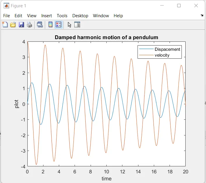
Angular Displacement and Angular Velocity plots were generated for a time range of 20 secs.

Error occured,

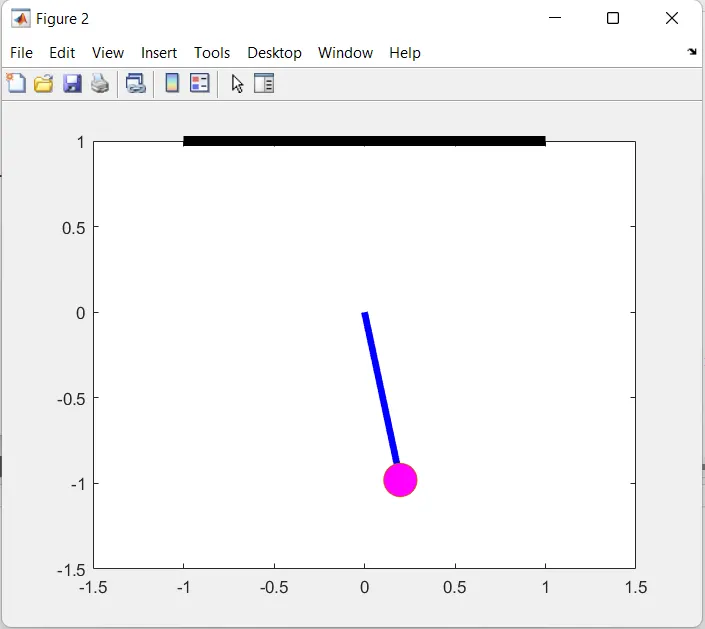
During creating the base of the pendulum, in the plot command co-ordinate was given wrong, then it is corrected to origin and then the error was fixed.

Link of the simple pendulum animation video,

https://youtu.be/W-58CpQeSBo