Week 3 - Solving second order ODEs

Solving 2nd order ODE's

Aim:

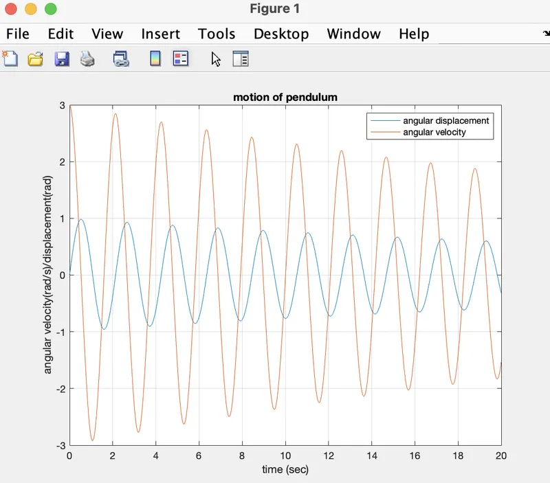
To write a program that solves the equation of motion of a simple pendulum with damping.

Theory:

A 2nd order differential cut and dried equation is which, any derivatives apropos of the free-spirited variable have order number greater than 2.

Simple-pendulum:

an ideal pendulum consisting of a point mass suspended by a trivial inextensible perfectly flexible thread and free to vibrate without friction.

the way pendulum moves depends on the newton's 2nd law,

Newton's second law of motion pertains to the behavior of objects for which all existing forces are not balanced. The second law states that the acceleration of an object is dependent upon two variables, the net-force acting upon the object and the mass of the object. The acceleration of an object depends directly upon the net force acting upon the object, and inversely upon the mass of the object. As the force acting upon an object is increased, the acceleration of the object is increased. As the mass of an object is increased, the acceleration of the object is decreased.

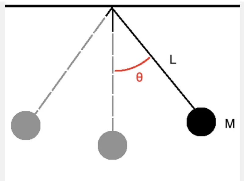
mathematical equation:

where,

b= damping

m= mass of the bob (kg)

g= acceleration due to gravity (m/s^2)

l= length of the string (m)

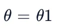
by substituting ,

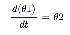
by solving the above equation we get,

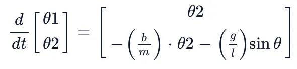
Coding:

calling function

function [dtheta_dt] = ode_func(t,theta,b,g,l,m)

theta1 = theta(1);

theta2 = theta(2);

dtheta1_dt = theta(2);

dtheta2_dt = -(b/m)*theta2 - (g/l)*sin(theta1);

dtheta_dt = [dtheta1_dt; dtheta2_dt];

end

%program for simple pendulum using ode45.

clear all

close all

clc

%input variables for the second order ode of a simple pendulum

b = 0.05;

g = 9.81;

l = 1;

m = 1;

%initial condition

theta_0 = [0; 3];

%time points

t_span = linspace(0,20,500);

%to solve second order ode.

[t,results] = ode45(@(t,theta) ode_func(t,theta,b,g,l,m),t_span, theta_0 );

%plotting of angular velocity and angular displacement

figure(1)

plot(t,results(:,1))

hold on

plot(t,results(:,2))

grid on

title('motion of pendulum')

xlabel('time (sec)')

ylabel('angular velocity(rad/s)/displacement(rad)')

legend('angular displacement','angular velocity')

hold off

angle = results(:,1);

%count command for iterations

ct = 1;

for j = 1 : length(angle)

alpha = angle(j);

figure(2)

title('motion of pendulum')

%fixed corordinates of one end of simple pendulum.

x0 = 0;

y0 = 0;

%moving coordinates of the bob.

x1 = l*sin(results(j,1));

y1 = -l*cos(results(j,1));

plot([x0 x1],[y0 y1],'linewidth',3,'color','r');

hold on;

plot([-1 1],[0 0],'linewidth',2,'color','b');

plot(x1,y1,'.','markersize',30);

axis([-1 1 -1 1])

hold off;

M(ct) = getframe(gcf);

ct = ct+1;

end

Program explanation:

Clear all, close all, clc are used to clear the work space, to clear the graphs that’s exists, and clear the command window.

The inputs are for the simple pendulum are specified and the b = damping coefficient = 0.05 (n-m/s), g = acceleration due to gravity = 9.81 (m/s), l = length of the string = 1(m), m = mass of the bob = 1 (kg).

t_span is a command used in the ode45 solver which specifies the time span of the iterations that are going to solve the ordinary differential equation.

graph:

animation:

animation of the coding is attached below.

Screen Recording 2022-07-16 at 11.10.35 PM

conclusion:

We have animated the simple pendulum using the ode45 solver where the second order is reduced to a simple differential equation where it is easy to solve the given equation.

The animation is made using the different points of the bob and the motion of the simple pendulum is created.