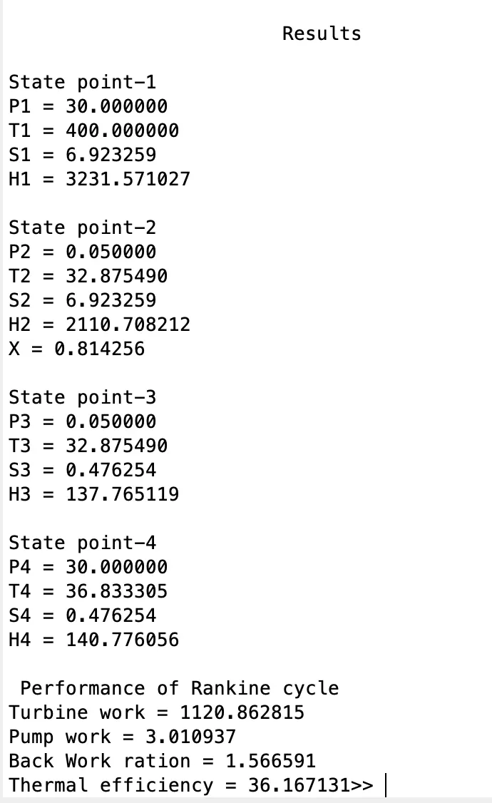
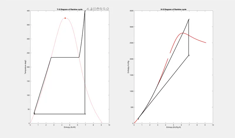
To create a program that simulates the state points of a rankine cycle from the inputs by user ad calculates the peformance parameters such as thermal efficiency, Back work ratio, turbine and pump work.
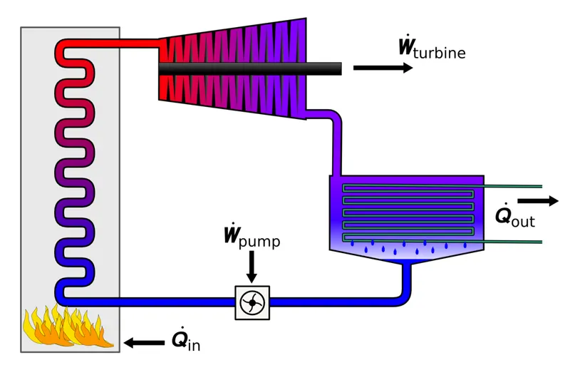
The Rankine cycle or Rankine vapour cycle is the process widely used for coal fired power plants or neuclear powerplants.In this the fuel is used to produce heat in the boiler that converts water to steam at high temperature and pressure which inturn drives the steam turbine.
Since water is used as the working fluid the efficiency of rankine cycle is limited due to the high heat of vapourization of water. The working fluid is to be recycled and reused constantly.
Command:
%% Rankine Cycle Simulator
%%
% Program to find the thermal efficiency, back work ratio and the state
% points of the rankine cycle
clear all
close all
clc
% inputs for calculating Rankine cycle
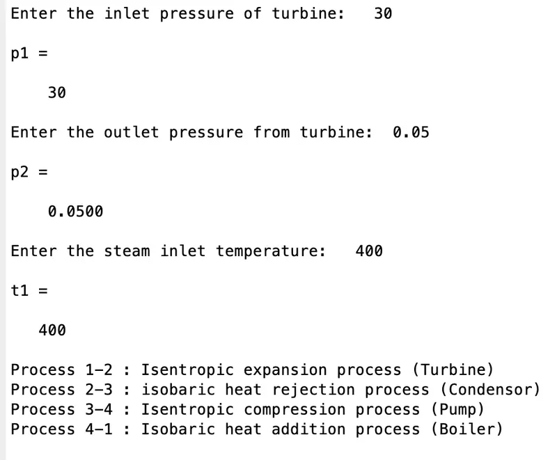
p1 = input('Enter the inlet pressure of turbine: ')
p2 = input('Enter the outlet pressure from turbine: ')
t1 = input('Enter the steam inlet temperature: ')
% pressure of state points
p4 = p1;
p3 = p2;
% Cycle information
fprintf('Process 1-2 : Isentropic expansion process (Turbine)\n')
fprintf('Process 2-3 : isobaric heat rejection process (Condensor)\n')
fprintf('Process 3-4 : Isentropic compression process (Pump)\n')
fprintf('Process 4-1 : Isobaric heat addition process (Boiler)\n')
%calculating the dryness fraction of state points
s1 = XSteam('s_pT',p1,t1); % state point 1
s2 = s1; % state point 2
sf2 = XSteam('sL_p',p2);
sg2 = XSteam('sV_p',p2);
sfg2 = sg2 - sf2;
x2 = (s1 - sf2)/sfg2;
if (x2 > 1)
t2 = XSteam('T_ps',p2,s2);
t_2 = XSteam('Tsat_p',p2);
t3 = t_2;
Td = linspace(t2,t_2,50);
s_2 = XSteam('sV_T',t_2);
s3 = XSteam('sL_T',t3);
s4 = s3;
else
t2 = XSteam('Tsat_p',p2);
t_2 = t2;
t3 = t2;
s3 = sf2; % State pont 3
s4 = s3; % state point 4
end
%calculating the enthalpy of state points
h1 = XSteam('h_pT',p1,t1); % state point 1
hf2 = XSteam('hL_p',p2); % state point 2
hg2 = XSteam('hV_p',p2);
hfg2 = hg2 - hf2;
h2 = hf2 + x2*hfg2;
h3 = hf2; % state point 3
v3 = XSteam('vL_p',p3); %specific volume
h4 = v3*(p1-p2)*100 + h3; % state point 4
cp = XSteam('Cp_ps',p3,s3);
cv = XSteam('Cv_ps',p3,s3);
k = 1 - (cv/cp);
t4 = t3*((p4/p3)^k);
t5 = XSteam('Tsat_p',p1);
t6 = t5;
s5 = XSteam('sL_T',t5);
s6 = XSteam('sV_T',t6);
% Turbine work
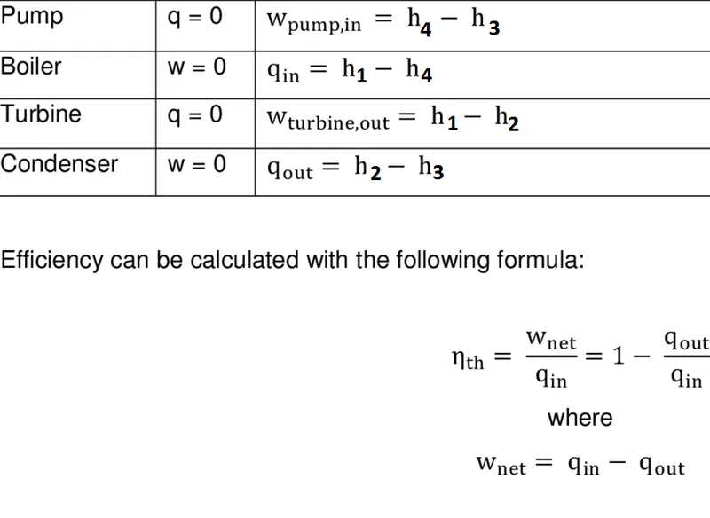
Wd_tb = h1 - h2;
% Pump work
Wd_pm = h4 - h3;
% Net work, Back work ratio and thermal efficiency of Rankine cycle
W_net = Wd_tb - Wd_pm;
bwr = (h1 - h4)/(h2 - h3);
efficiency = W_net/(h1-h4);
efficiency = efficiency*100;
% state point 1 parameters
fprintf('\n\t\t\tResults\n')
fprintf('\nState point-1')
fprintf('\nP1 = %f',p1)
fprintf('\nT1 = %f',t1)
fprintf('\nS1 = %f',s1)
fprintf('\nH1 = %f',h1)
% state point 2 parameters
fprintf('\n\nState point-2')
fprintf('\nP2 = %f',p2)
fprintf('\nT2 = %f',t2)
fprintf('\nS2 = %f',s2)
fprintf('\nH2 = %f',h2)
fprintf('\nX = %f',x2)
% state point 3 parameters
fprintf('\n\nState point-3')
fprintf('\nP3 = %f',p3)
fprintf('\nT3 = %f',t3)
fprintf('\nS3 = %f',s3)
fprintf('\nH3 = %f',h3)
% state point 4 parameters
fprintf('\n\nState point-4')
fprintf('\nP4 = %f',p4)
fprintf('\nT4 = %f',t4)
fprintf('\nS4 = %f',s4)
fprintf('\nH4 = %f',h4)
% Performance parameters of Rankine cycle
fprintf('\n\n Performance of Rankine cycle')
fprintf('\nTurbine work = %f',Wd_tb)
fprintf('\nPump work = %f',Wd_pm)
fprintf('\nBack Work ration = %f',bwr)
fprintf('\nThermal efficiency = %f',efficiency)
%plotting of the graph
% Data - boiler sensible heat addition at superheated condition
T = linspace(t6,t1,500);
for i = 1:length(T)
S(i) = XSteam('s_pT',p1,T(i));
H(i) = XSteam('h_pT',p1,T(i));
end
% Data - saturation temperature curve
maxt = linspace(1,t1,500);
for j = 1:length(maxt)
satlS(j) = XSteam('sL_T',maxt(j));
satvS(j) = XSteam('sV_T',maxt(j));
satlH(j) = XSteam('hL_T',maxt(j));
satvH(j) = XSteam('hV_T',maxt(j));
end
%%
%% T-S Diagram for Rankine cycle
subplot(1,2,1)
% plot - saturation curves
plot(satlS,maxt,'color','r')% saturation liquid temperatures
hold on
plot(satvS,maxt,'color','r')% saturation vapour temperatures
plot(4.4230,373.6,'o','MarkerFaceColor','r','MarkerSize',7) % critical temperature
%plot - Curve for points t5 and t6
line([s5 s6],[t5 t6],'Color','k','lineWidth',2)
%plot - Curve for points t6 and t1
plot(S,T,'Color','k','lineWidth',2)
%plot - Curve for points t1 and t2
line([s1 s2],[t1 t2],'Color','k','lineWidth',2)
if (x2 > 1)
% Data - constant pressure curve at boiler inlet if present
for i = 1:length(Td)
Sd(i) = XSteam('s_pT',p2,Td(i));
Hd(i) = XSteam('h_pT',p2,Td(i));
end
%plot - Curve for points t2 and t_2 (if present)
plot(Sd,Td,'color','k','lineWidth',2)
% plot - line for t_2 and t3 (if present)
line([s_2 s3],[t_2 t3],'Color','k','lineWidth',2)
else
line([s2 s3],[t2 t3],'color','k','lineWidth',2)
end
%plot - Curve for points t3 and t4
line([s3 s4],[t3 t4],'Color','k','lineWidth',2)
% plot - Constant pressure heat addition curve till saturation liquid line
line([s4 s5],[t4 t5],'Color','k','lineWidth',2)
% labelling of graph
title('T-S Diagram of Rankine cycle')
xlabel('Entropy (KJ/K)')
ylabel('Temprature degC')
% Marking the state points
text(s1,t1,"1");
text(s2,t2,"2");
if (x2 > 1)
text(s_2,t_2,"2'");
end
text(s3,t3,"3");
text(s4,t4,"4");
%% H-S diagram for rankine cycle
subplot(1,2,2)
% plot for saturation curves of liquid and vapuor
plot(satlS,satlH,'color','r','lineWidth',2)
hold on
plot(satvS,satvH,'color','r','lineWidth',2)
% plot - isentropic expansion line
line([s1 s2],[h1 h2],'color','k','lineWidth',2)
if (x2 > 1)
h_2 = XSteam('h_ps',p2,s_2);
%plot - constant pressure heat addition ,if outlet steam is superheatedcond.
plot(Sd,Hd,'color','k','lineWidth',2)
% Data - constant pressure heat rejection curve enthalpy values
entrpy = linspace(s_2,s3,100);
for k = 1:length(entrpy);
enthlpy(k) = XSteam('h_ps',p2,entrpy(k));
end
% Plot - constant pressure heat rejection curve
plot(entrpy,enthlpy,'color','k','lineWidth',2)
else
% Data - constant pressure heat rejection curve enthalpy values if
% steam is wet or dry saturated vapour
entrpy = linspace(s2,s3,100);
for k = 1:length(entrpy);
enthlpy(k) = XSteam('h_ps',p2,entrpy(k));
end
% Plot - constant pressure heat rejection curve
plot(entrpy,enthlpy,'color','k','lineWidth',2)
end
%plot - Isentropic compression line
line([s3 s4],[h3 h4],'color','k','lineWidth',2)
% data - Constant pressure heat addition curve enthalpy values
entrpy1 = linspace(s4,s1,100);
for l = 1:length(entrpy1)
enthlpy1(l) = XSteam('h_ps',p1,entrpy1(l));
end
% plot - Constant pressure heat addition curve
plot(entrpy1,enthlpy1,'color','k','lineWidth',2)
% labelling of graph
title('H-S Diagram of Rankine cycle')
xlabel('Entropy (KJ/Kg K)')
ylabel('Enthalpy KJ/Kg')
% Marking the state points
text(s1,h1,"1");
text(s2,h2,"2");
if (x2 > 1)
text(s_2,h_2,"2'");
end
text(s3,h3,"3");
text(s4,h4,"4");
%%
Multiple errors were encountered during the coding process and mainly was occured due to invalid syntaxes or other function calling statments.
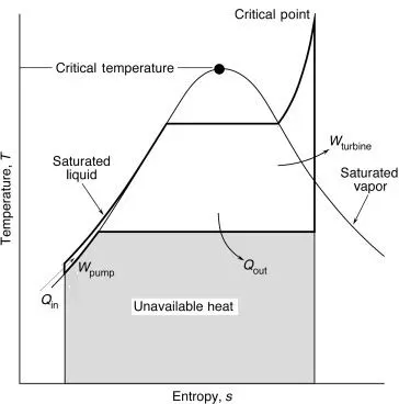
A code to simulate the Rankine cycle is done with calculation for performance parameters along with plots for T-S and H-S diagram.