Week 3 - Solving second order ODEs

Aim: Writing a Matlab code to solve ODE and to show the animation of pendulum motion using Matlab.

Solution: Here, ODE equation given is as follows

in Order to solve this, lets assume that

theta = theta1

hence, dtheta/dt = dtheta1/dt = theta2.....(1)

Also, dtheta^2/dt = dtheta1^2/dt^2 = d/dt(dtheta1/dt) = dtheta2/dt.....(2)

Now substituting these values in in ODE equation, we get

dtheta2/dt + (b/m)theta2 + (g/l)sin(theta2) = 0

Solving by subsititution, we get

d/dt[theta1;theta2] = [theta2; -(b/m)theta2 - (g/l)sin(theta1)]

Code:

In order to solve using Matlab, we need to first define a function that can be called to solve the ODE. The function code is as follows

function [dtheta_dt] = ode_func(t,theta,b,g,l,m)

theta1 = theta(1)
theta2 = theta(2)
dtheta1_dt = theta2
dtheta2_dt = -(b/m)*theta2 -(g/l)*sin(theta1)
dtheta_dt = [dtheta1_dt;dtheta2_dt]

end

Here we are defining theta as the function of several variables like time, and then solving the ODE as shown previously to get the solution easily.

We will call this function in the main code, which is as follows.

clear all
close all
clc

b = 0.05
g = 9.81
l = 1
m = 1

%Initial condition of angular displacement and angular velocity

theta_0 = [0;3]

% time points, taking as 20 seconds
t_span = linspace(0,20,300)

%solve ODE
[t,results] = ode45(@(t,theta) ode_func(t, theta, b,g,l,m),t_span,theta_0)

%plotting
figure(1)

hold on
plot(t,results(:,1))
plot(t,results(:,2))
title('Motion of Pendulum')
legend('Angular displacement','Angular velocity')
xlabel('plot')
ylabel('time (sec)')
grid on
%animation
%using for loop to get the position of pendulum at a particular
%velocity and time.

ct=1
for i = 1:length(results(:,1))
    x_initial = 0
    y_initial = 0
    
    x_final = l*sin(results(i,1))
    y_final = -l*cos(results(i,1))
    
    %plot for animation
    figure(2)
    plot([-0.5 0.5],[0 0 ], 'linewidth',4)
    hold on
    plot([x_initial x_final],[y_initial y_final],'linewidth',2)
    
    
    plot([x_final x_final],[y_final y_final],'O','markersize',15,'markerfacecolor','r')
    axis([-1.5 1.5 -1.5 1])
    pause(0.03)
    M(ct)= getframe(gcf)
    ct=ct+1
    hold off
    
end 

%movie

movie(M)
videofile = VideoWriter('Animation of Pendulum','MPEG-4')
open(videofile)
writeVideo(videofile,M)
close(videofile)

1.We start the code using clear all, close all, close all, clc.

2.We now define inputs and variables like damping coefficient, gravity, mass of the ball, length of the string.

3. Then we define timespan, angular velocity and angular displacement. and use inbuilt ODE solver in Matlab i.e. ODE45, which gives us an output [t,results], which means that results have been claculated with respect to time.

4. Using the results, a graph is plotted, having angular displacement w.r.t time and angular velocity w.r.t. time. The graph is as shown.

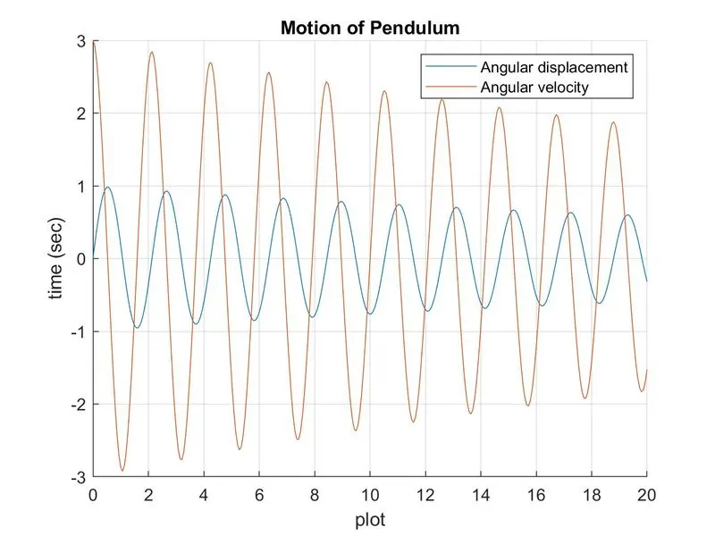
Now we use for loop to get the frame for each time interval in order to get the animation. The movie is made using movie command, VideoWriter command to assign the video format, open command to open the video and writevideo command is used to plot the frames, with close command to close the video file.

Animation Video Link: https://youtu.be/VuyNT3Mu7Io