Matlab code to create PV diagram for Otto cycle and to find its thermal efficiency.

Objective: To write a Matlab code for otto cycle and show plot of the PV diagram. We also need to find its therml efficiency.

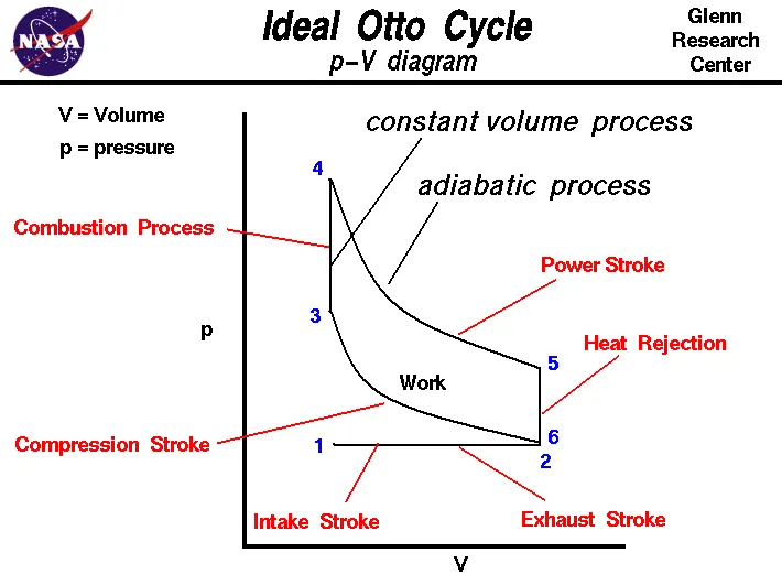
Solution An otto cycle describes the combustion process taking place in a spark ignition piston engine, showing the various thermodynamic processes involved in it. The fuel used here is petrol. The following diagram shows the otto cycle processes.

In Otto cycle, there are two types of processes taking place.

1. Isentropic compression (from 2-3) and isentropic expansion (from 4-5). its formula is PV^gamma = C

2. Isochoric heat addition(from 3-4) and isochoric heat rejection (from 5-6).

To find the instantaneous change of pressure and volume during the process, we will use the following formula.

(V/Vc) = 1 + (1/2)(cr-1)(R + 1-cos(theta)-sqrt(R^2 - sin(theta)^2))

3. Thermal efficiency is given by 1 - (1/cr^(gamma-1))

4. The unit of pressure is 'Pascal (Pa)'. volume is in m^3, temperature in Kelivin (K).

5. Compression Ratio is given by (v_s+v_c)/v_c, where v_s is swept volume and v_c is clearance volume.

Procedure:

1. Assuming pressure at starting p1 to be 101325 Pa and initial temperature t1 be 500K. Also we define various engine parameters like bore dia, stroke length, compression ratio, connecting rod and gamma.

2. For state 2, using the formula pv^gamma = constant, we determine the values of p2 and t2. The values of swept volume and clearance volume are calculated using the following formula

v_s = (pi/4)*bore^2*stroke
v_c = v_s/(cr-1)

3. Temperature at state 3 is assumed to be 2300K and pressure is calculated using ideal gas equation PV/T constant. Here v3=v2 (Constant volume heat addition.)

4. We gain use the formula in step 2. to determine tempertaure and pressure for the process 3 to 4 i.e isentropic expansion.

The we use the plot command to plot the points obtained from above 4 procedures. But in order to get the proper PV diagram, we need to find the instantaneous volume and pressure during the combustion process.

5. We use the 'Function' command to make a separate matlab function, that can be called in the main program in order to determine the instantaneous volume and pressure during compressiona and expansion stroke.

following is the function program

function V = piston_kinematics(bore,stroke,connecting_rod,cr,start_crank,end_crank)

% inputs
a = stroke/2
R = connecting_rod/a


v_s = (pi/4)*bore^2*stroke
v_c = v_s/(cr-1)

theta = linspace(start_crank,end_crank,100)

term1 = (cr-1)*0.5
term2 = R+1-cosd(theta)
term3 = (R^2-sind(theta).^2).^0.5

V = (1 + term1*(term2-term3)).*v_c

end

This function is called upon as shown in the following code sample for compression stroke.

% parameters at state 2!
v2 = v_c
% we know for isentropic process, PV^gamma is constant
% p1*v1^gamma = p2*v2^gamma
%p2 = p1*v1^gamma/v2^gamma
p2 = p1*cr^gamma

%using ideal gas equation to determine temperature
%p1v1/t1 = p2v2/t2
t2 = p2*v2*t1/(p1*v1)


V_compression = piston_kinematics(bore,stroke,connecting_rod,cr,180,0)
const_c = p1*v1^gamma
P_compression = const_c./V_compression.^gamma

for expansion stroke

% parameters at state 3
v3 = v2
%p2v2/t2 = p3v3/t3
p3 = (p2*t3)/t2

V_expansion = piston_kinematics(bore,stroke,connecting_rod,cr,0,180)
const_c = p3*v3^gamma
P_expansion = const_c./V_expansion.^gamma

These points are also added to the main code in order to get the desired PV diagram.

The Main Code is as follows

clear all
close all
clc

%Engine parameters
bore = 0.1       
stroke = 0.1
connecting_rod = 0.15
%compression ratio
cr = 12
gamma = 1.4

%State Variables, Pressure in Pa and temperature in K
p1 = 101325
t1 = 500
t3 = 2300

%calculations of swept volume v_s and clearance volume v_c, in m^3
v_s = (pi/4)*bore^2*stroke
v_c = v_s./(cr-1)

%volume at start of compression stroke v1
v1 = v_s+v_c


% parameters at state 2!
v2 = v_c
% we know for isentropic process, PV^gamma is constant
% p1*v1^gamma = p2*v2^gamma
%p2 = p1*v1^gamma/v2^gamma
p2 = p1*cr^gamma

%using ideal gas equation to determine temperature
%p1v1/t1 = p2v2/t2
t2 = p2*v2*t1/(p1*v1)


V_compression = piston_kinematics(bore,stroke,connecting_rod,cr,180,0)
const_c = p1*v1^gamma
P_compression = const_c./V_compression.^gamma


% parameters at state 3
v3 = v2
%p2v2/t2 = p3v3/t3
p3 = (p2*t3)/t2

V_expansion = piston_kinematics(bore,stroke,connecting_rod,cr,0,180)
const_c = p3*v3^gamma
P_expansion = const_c./V_expansion.^gamma


%parameters at state 4
v4 = v1
%p3v3^gamma = p4v4^gamma
p4 = p3*(v3/v4)^gamma
t4 = (p4*v4*t3)/(p3*v3)


%Thermal Efficiency
efficiency = (1-1/cr^(gamma-1))*100


%Plotting the otto cycle!

hold on
plot(v1,p1,'d','color','r')
plot(V_compression,P_compression)

plot(v2,p2,'d','color','g')
plot([v2 v3],[p2 p3],'color','k')

plot(v3,p3,'d','color','m')
plot(V_expansion,P_expansion)

plot(v4,p4,'d','color','b')
plot([v4 v1],[p4 p1],'color','k')

xlabel('Volume m^3')
ylabel('Pressure Pa')
legend('State1','Isentropic compression','State2','isochoric heat addition','State3','isentropic expansion','Satet4','isochoric heat rejection')
title('Otto cycle')

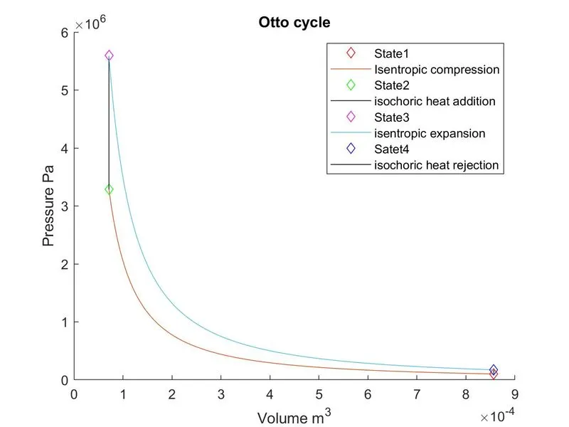
Following is the PV diagram of Otto Cycle.

Thermal Efficiency from command window

t4 =

  851.2465


efficiency =

   62.9893

Result:

1. The code executed successfully and PV diagram for Otto Cycle was obtained.

2. Thermal Efficiency obtained was 62.98%

3. The errors were typo errors and hence were corrected with proper inspection of the code.