Solving second order ODEs for a simple pendulum
Report on : Matlab to simulate the motion of a simple pendulum.
Video Link(Youtube):- https://youtu.be/NhTKuXoJHcU
Aim:- 1.Write a program in MATLAB that can solve 2nd order ODE for a simple pendulum and simulate the the pendulum motion.
Objectives:- 1.write a program that solves the following ODE for a simple pendulum.
2. Create an animation of the motion of the pendulum, similar to figure shown below.
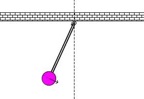
Theory:-
The simple pendulum is another mechanical system that moves in an oscillatory motion. It consists of a point mass ‘m’ suspended by means of light inextensible string of length L from a fixed support as shown in Fig.2. The motion occurs in a vertical plane and is driven by a gravitational force. The forces which are acting on the mass are shown in the figure. The tangential component of the gravitational force, mg sin θ, always acts towards the mean position θ = 0 opposite to the displacement, restoring force acting tangent to the arc.
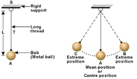
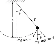
fig. 1 fig. 2
Since the period is independent of the mass, a pendulum of equal length at the same location oscillates with equal periods. The analogy between the simple pendulum is the mass–spring system as shown in Fig.3. The displacement, velocity, acceleration, kinetic energy and potential energy.
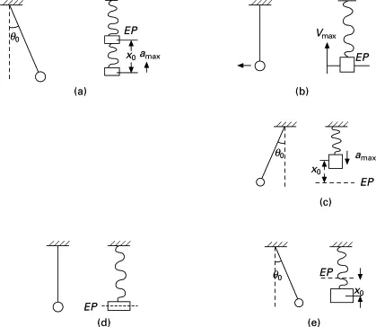
fig. 3
The way the pendulum moves depends on the Newtons second law. When this law is written down, we get a second order Ordinary Differential Equation that describes the position of the "ball" w.r.t time.
In Engineering, ODE is used to describe the transient behavior of a system.
Similarly, there are hundreds of ODEs that describe key phenomena and if you have the ability to solve these equations then you will be able to simulate any of theses systems.
In the above equation,
- g = gravity in m/s2,
- L = length of the pendulum in m,
- m = mass of the ball in kg,
- b=damping coefficient.
To solve this second order ODE, we split the equation into first order ODEs:
given,
 ....Eq.1
Let,

then,

&
 ....Eq.2
then Eq.1 becomes

so,
 ....Eq.3
we can also write (Eq.2) and (Eq.3) as
 ....Eq.4
Now the (Eq.4) is modified into a matrix form.
MATLAB code to solve the given ode equation :-
% Matlab script to solve 2nd order ODE for a simple pendulam using MATLAB:
% Plot an animation for the motion of a simple pendulam using MATLAB:


clear all              % to clear all the previous written code
close all              % to close all the previously opened plots
clc                    % to clear the workspace window

% inputs
                        % where-
b= 0.05;                % b=dampping coefficient
g =9.81;                % g=accl. due to gravity(m/s^2)
l= 1;                   % l=length of the string (m)
m= 1;                   % m = mass (kg)

% Initial condition for a simple pendulam:

theta_0 = [0,5];        % where-
                        % '0' is the value taken for initial displacement
                        % '5' is the value taken for intial velocity

t_span = linspace(0,20,500);
                        % time span from 0 to 10 sec. and values taken are 500


% For solving ODE by calling function:(using ode45 inbuilt solver in MATLAB)

[t, results] = ode45(@(t,theta) ode_func(t,theta,b,g,l,m),t_span, theta_0);


% Plotting:

figure(1)

hold on
plot(t,results(:,1))      % displacemnt vs. time plot.
plot(t,results(:,2))      % velocity vs. time plot.
xlabel('time')            % time is taken on x axis
ylabel('plots')           % displacement and velocity is taken on x axis
legend('displacement','angular velocity')
grid on


% plotting an animation of a simple pendulum:

ct=1;
x0=10;                       % where:
y0=10;                       % x0,y0 be the fixed point where pendulum is attached
THETA_1=results(:,1);        % THETA_1 :linear displacement of pendulum from its mean postion

for i =1:length(results(:,1))     % for loop is used to get all the displacement values

    THETA_2=THETA_1(i)       % THETA_2 :angular deviation of pendulum from its mean position
    x1=10+(3*sin(THETA_2))   % x1,y1 be the position of mass(bob) attached to the string.
    y1=5-(3*cos(THETA_2))    % to get 3 times more maginfication x and y are muliplied by 3


figure(2)
                                              % positions:
plot(x0,y0,'*','color','k')                   % fixed point where string is attached.
hold on
plot(x1,y1,'O','color','r',Linewidth=15)      % bob attached to the either end of string.
plot([x0 x1],[y0 y1],'color','b',LineWidth=2) % string plot on a graph.
hold off
axis([5 15 0 15])                             % range values for x axis and y axis.

M(ct) = getframe(gcf);                        % all the frames of plots are stored in array 'M'.
ct=ct+1;
end


% Creating a movie showing the current animation for a simple pendulum:


movie(M)                % MATLAB will generate a movie by taking frames through matrix called 'M'

videofile = VideoWriter('simple_pendulum.avi','Uncompressed AVI')
                        % videofile of .avi (extension)is created and stored by using Videowriter command
                        % file name also assigned as 'simple_pendulum'.

open(videofile)         % MATLAB will opens the videofile
writeVideo(videofile,M) % MATLAB will write the given video file by using given command instruction.
                        % MATLAB will auto play the video.
close(videofile)        % MATLAB will automatically close the videofile as it finishes.
Output:-
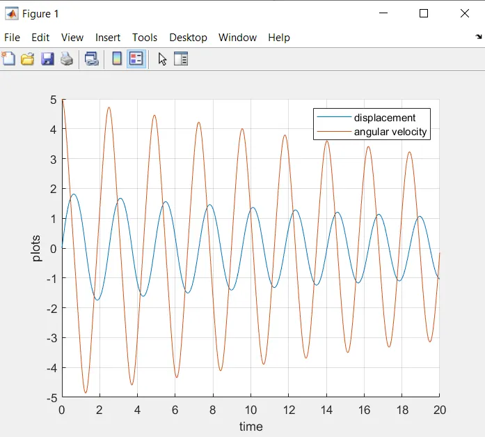
Above fig. shows how displacement and velocity is varing w.r. t for a given simple pendulum. We can say that both velocity and displacement is a function of time. and the motion plot obtain is SHM.
ERRORS faced and methods of error elimination:-
ERROR 01: not using 'hold on' command: fixed point plot and bob is not showing as MATLAB executiing the last plot only
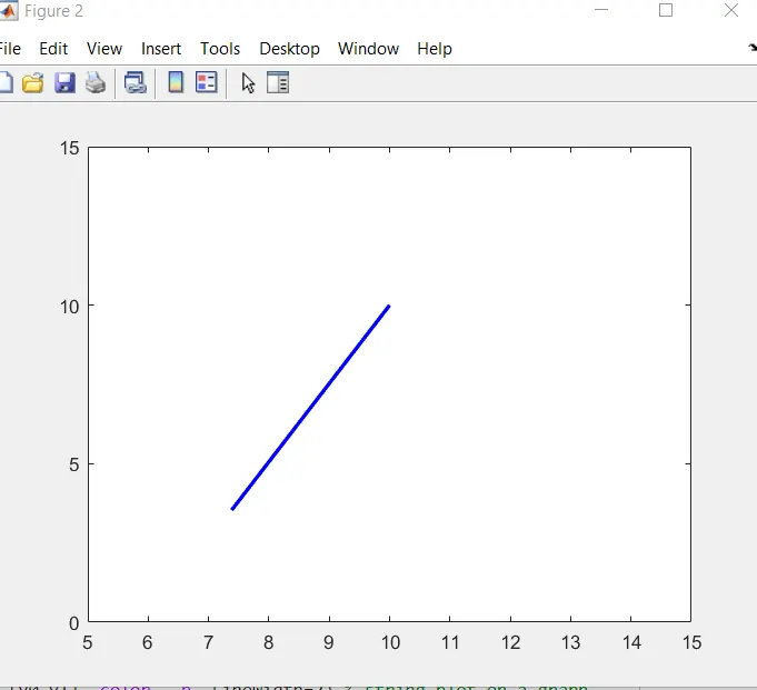
the error gets eliminated just by adding hold on command before the plots which we want to keep and overwrite.
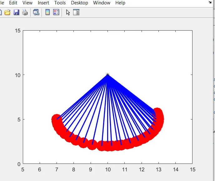
the error gets eliminated just by adding hold off command after the plots which we dont want to keep and overwrite.
- A MATLAB code for a given pendulum ODE equation is compiled and run succesfully.
- A movie IS created showing the simulation of motion for a given simple pendulum.
- A report is created and submitted at skill lync.project :https://skill-lync.com/student-projects/matlab-to-solve-2nd-order-ode-for-simple-pendulum-and-simulate-the-motion-of-a-simple-pendulum
Referances:-
- Course on Matlab for mechanical -Skill lync.
- Books: Theory of machines by 'S. S. Rattan' and Mechanical vibration by 'G K Grover'
- Softwares:Mathworks-Matlab and Octave