Otto Cycle using MATLAB -(Finding the thermal efficiency and plotting a graph of a PV diagram using MATLAB).

Aim: Write a program in MATLAB that can solve Otto Cycle and make a plot of it.

Objectives:-

1. Plot P-V diagram for a given otto cycle

2. Calculating thermal efficiency for a given Otto Cycle.

Theory:-

An Otto cycle is an idealized thermodynamic cycle that describes the functioning of a typical spark ignition piston engine. It is the thermodynamic cycle most commonly found in automobile engines.

Fig 1: PV diagram Fig 2 : TS diagram

• Process 0–1: A mass of air is drawn into piston/cylinder arrangement at constant pressure.
• Process 1–2: An adiabatic (isentropic) compression of the charge as the piston moves from bottom dead center (BDC) to top dead center (TDC).
• Process 2–3: A constant-volume heat transfer to the working gas from an external source while the piston is at top dead center. This process is intended to represent the ignition of the fuel-air mixture and the subsequent rapid burning.
• Process 3–4: An adiabatic (isentropic) expansion (power stroke).
• Process 4–1: Completes the cycle by a constant-volume process in which heat is rejected from the air while the piston is at bottom dead center.
• Process 1–0: The mass of air is released to the atmosphere in a constant pressure process.

Governing Equations:

• Ideal Gas Equation: P1V1/T1 = P2V2/T2 from (PV=nRT)

• Thermal Efficiency:

• Change of volume inside engine combustion chamber:

Procedure:

Otto Cycle plot using MATLAB code (constant slopes during compression and expansion):(line by line explaination using comments)

• Initial Otto Cycle Plot using MATLAB:-

% otto cycle-using matlab (theoretical plot)


clear all           %to clear all the script window
close all           %to clear all previous plots
clc                 % to clear workspace window


%Inputs

gamma=1.4            % Ratio Of Specific Heat Constants(gamma=Cp/Cv)              
t3=2300              % Temperature before start of expansion (K)


% state variable at state pt.1


p1=101325           % Pressure before start of compression (Pa)
t1=500              % Temperature before start of compression (K)


%engine geometric parameter


bore=0.1                     % Bore diameter (m)
stroke=0.1                   % Stroke length (m)
con_rod=0.15                 % Connecting rod length (m)
cr=12                        % Compression ratio



%calculating the swept volume and clearance volume


v_s=(pi/4)*bore^2*stroke;           % Swept volume (m^3)                                 
v_c=v_s/(cr-1);                     % Clearance volume (m^3)
v1= v_s+v_c                         % Volume before start of compression (m^3)
v2=v_c                              % Volume at the end of compression (m^3)



%state variable at pt.2 | p2v2^gamma=p1v1^gamma ( By using ideal gas equation)
%p2=p1(v1/v2)^gamma=p1*v1^gamma                                 
p2= p1*cr^gamma                   % Pressure at the end of compression (Pa)                                           
% p1v1/t1=p2v2/t2(ideal gas equation)
t2= p2*v2*t1/(p1*v1)              % Temperature at the end of compression (K)





%state variable at state pt. 3 
v3=v2                                % Constant volume process
%p3v3/t3=p2v2/t2 | p3= p2*t3/t2 ( By using ideal gas equation)
p3= p2*(t3/t2)                       % Pressure before expansion(Pa)




%state variable at state pt. 4
v4=v1                                       % Constant volume process
%p3v3^gamma = p4v4^gamma | p4 = p3(v3/v4)^gamma (By using ideal gas equation)
p4 = p3*(v3/v4)^gamma                       % Pressure at the end of expansion (Pa)


% Plotting (state points and processes ) 
figure(1)
hold on                                  %to get all plots in same fig. window
plot(v1,p1,'*','Color','r')              % state point 1
plot(v2,p2,'*','Color','r')              % state point 2
plot(v3,p3,'*','Color','r')              % state point 3
plot(v4,p4,'*','Color','r')              % state point 4
plot ([v1 v2 v3 v4 v1],[p1 p2 p3 p4 p1],'color','b')       % all process plots

• Initial Otto Cycle Plot using octave:

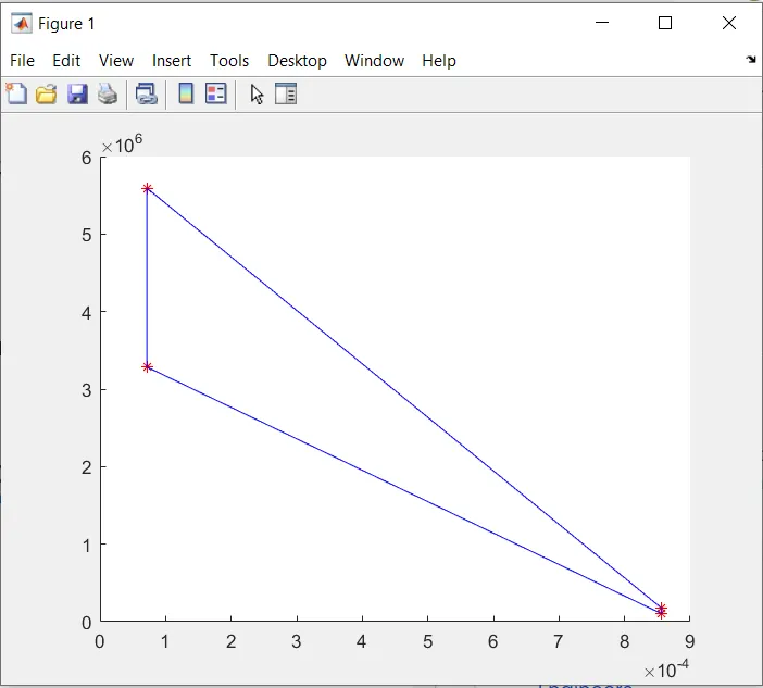
From the above plot it is found that process 1-2 & 3-4 are of constant slope but we know that during isentropic compression & isentropic expansion , pressure & volume changes from point to point. Therefore the above plot is not valid as Otto cycle has two isnetropic process having non linear slopes.

• process (1-2) : is an isentropic compression
• process (3-4) : is an isentropic expansion

To obtain Otto Cycle with correct assumption we need to find instantaneous changes in pressure & volume during process 1-2 & 3-4.

we can get those values by using function in MATLAB: finding volume and pressure at various points during isentropic compression and expansion. Using equation PV^gamma=constant ( reversible adiabatic process)

• Function used: A matlab code using function command :-

% Calculating the actual volume during isentropic process for otto cycle
% By using equation  V/v_c= 1+0.5(cr-1)[R+1-cosd(theta)-(r^2-sind(theta)^2]^0.5

function [V]= engine_kinematics(bore,stroke,con_rod,start_crank,end_crank)

%inputs

cr=12                                      % compression ratio
a= stroke/2                                % crank radius (m)
R=con_rod/a                                % obliquity ratio
theta=linspace(0,720,100)                  % 100 values of theta taken for 720 degree crank angle 

%spliiting above formula into multiple terms for the ease of calculation

term1= 0.5*(cr-1)
term2=R+1-cosd(theta)
term3=(R^2-sind(theta).^2).^0.5

%calculating the swept volume and clearance volume

v_s=(pi/4)*bore^2*stroke;   %swept volume (m^3)
v_c=v_s/(cr-1);             %clearance volume(m^3)

% V during isentropic process
V = (1+term1*(term2-term3)).*v_c

end

From the above function volume at different points (assumed 100 points) during isentropic compreesion process can be obtained

by using the governing equation where volume is a function of cranck angle (theta) when piston moves from BDC to TDC (180 to 0).

similarly we can get the values during isentropic expansion process w.r.t cranck angle (theta), when piston moves from TDC to BDC (0 to 180)

• Final Otto Cycle Plot using MATLAB (by calling above function):-

% script that can solve an otto cycle and make plots for it.

clear all           % clear all the previous written code
close all           % closes all the previous plots
clc                 % to delet all the workspace saved data


% required inputs

gamma=1.4                   % ratio of specific heats for otto cycle
p1=101325                   % pressure(Pa) at the start of compression
t1=500                      % temperature(K) at the start of compresssion
t3=2300                     % temperature(K) at the start of expansion


%engine geometric parameters


bore=0.1                                    % bore diameter (m)
stroke=0.2                                  % stroke length (m)
con_rod=0.15                                % connecting rod length(m)
cr=12                                       % compression ratio


% calculating the swept volume and clearance volume

v_s=(pi/4)*bore^2*stroke;                    % swept volume (m^3)
v_c=v_s/(cr-1);                              % clearance volume (m^3)


% state variable at state pt 1

v1= v_s+v_c                            % Volume before start of compression (m^3)
v2=v_c                                 % Volume at the end of compression (m^3)



%state variable at pt.2 | p2v2^gamma=p1v1^gamma
%p2=p1(v1/v2)^gamma=p1*v1^gamma (Ideal gas equation )
p2= p1*cr^gamma                          % Pressure at the end of compression (Pa)                                     
constant_c= p1*v1^gamma;

% Calling matlab function(engine_kinematics)
V_compression=engine_kinematics(0.1,0.2,0.15,180,0);            % Instataneous volume during compression
P_compression=constant_c./V_compression.^gamma;                 % Instataneous pressure during compression
t2= p2*v2*t1/(p1*v1) % from eq. p1v1/t1=p2v2/t2                 % Temperature at the end of compression (K)


%state variable at state pt. 3

v3=v2                                                             % Constant volume process
p3= p2*(t3/t2) % from eq. p3v3/t3=p2v2/t2
constant_c2= p3*v3^gamma
V_expansion=engine_kinematics(0.1,0.2,0.15,0,180)                 % Instataneous volume during expansion
P_expansion=constant_c2./V_expansion.^gamma                       % Instataneous pressure during expansion

%state variable at state pt. 4

v4=v1                                                             % Constant volume process 
p4 = p3*(v3/v4)^gamma%from eq. p3v3^gamma = p4v4^gamma         % Pressure at the end of expansion (Pa)
t4= p4*v4*t3/(p3*v3) %from eq. p3v3/t3=p4v4/t4                    % Temperature at the end of expansion (K)


% Calculating Thermal efficiency

Thermal_efficiency = 1-(1/(cr)^(gamma-1))


% plotting

hold on
plot(v1,p1,'*','Color','b')                             % State point 1 
plot(V_compression,P_compression,'Color','r')           % Process 1-2 (isentropic compression)
plot(v2,p2,'*','Color','b')                             % State point 2                             
plot([v2 v3],[p2 p3],'Color','r')                       % Process 2-3 (constant volume)
plot(v3,p3,'*','Color','b')                             % State point 3
plot(V_expansion,P_expansion,'Color','r')               % Process 3-4 (isentropic expansion)
plot(v4,p4,'*','Color','b')                             % State point 4
plot([v4 v1],[p4 p1],'Color','r')                       % Process 4-1 (constant volume)
xlabel('pressure(Pa)')
ylabel('Volume(m^3)')
grid on

• Final Otto Cycle Plot using octave:-

Output(thermal Efficiency):-

Conclusion:-

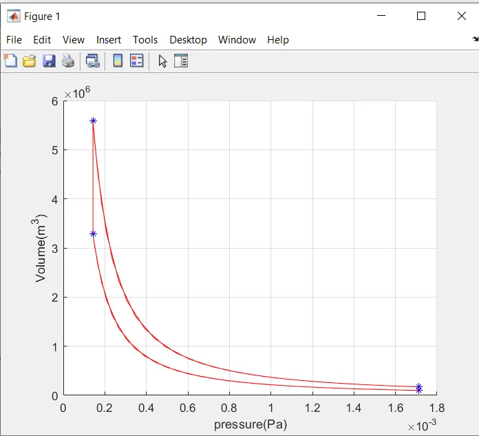
• The matlab code for an otto cycle is compiled and executed successfully.
• PV diagram for the given otto cycle plotted by taking assumption for an air standard cycle.
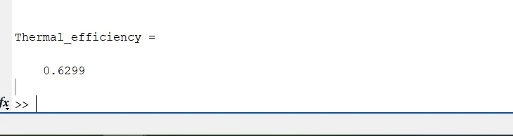
• Thermal efficiency for a given otto cycle is calculated and it is found to 0.6299 i.e 62.99%
• Hence, Air standard efficiency is depends upon compression ratio(cr) and gamma,
• Higher is the cr value more will be the efficiency but at very high cr value knocking occures so an optimum value of a compreesion ratio must be selected for better engine performance.

Referances:-

• Course on Matlab for mechanical -Skill lync.
• Books:1. I C Engine by Heywood, V.Ganesan, 2.Yunus A. Cengel and Boles, “Engineering Thermodynamics".
• Softwares:Mathworks-Matlab and Octave