Week 3 - Solving second order ODEs

AIM: Simulate the transit behaviour of the simple pendulum.

OBJECTIVE:

• To write a program that will simulate the pendulum motion by using MATLAB.
• To animate the motion of the pendulum

THEORY:

Simple Pendulum:

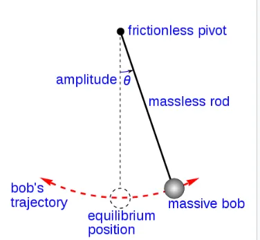
An ideal simple pendulum consists of a heavy point mass (called bob) tied to one end of a perfectly inextensible, flexible and weightless string. In practice, we make it by tying a metallic spherical bob to a fine cotton stitching thread.

A simple pendulum shows periodic motion, and it occurs in the vertical plane and is mainly driven by the gravitational force.

Length of a Simple Pendulum

The distance between the point of suspension of the pendulum and its Centre of Gravity (C.G.), which is the C.G. of the bob, is called the length of the simple pendulum. It is represented using the aphabet ( l ).

Time Period of a Simple Pendulum

Time period is the time taken by the bob of the simple pendulum to make one complete oscillation. It is represented by the letter T.

Formulas:

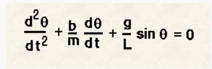
Where

b = Damping co-efficient

m = mass of the ball in kg

g = gravity in m/s^2

l = length of the pendulum in m

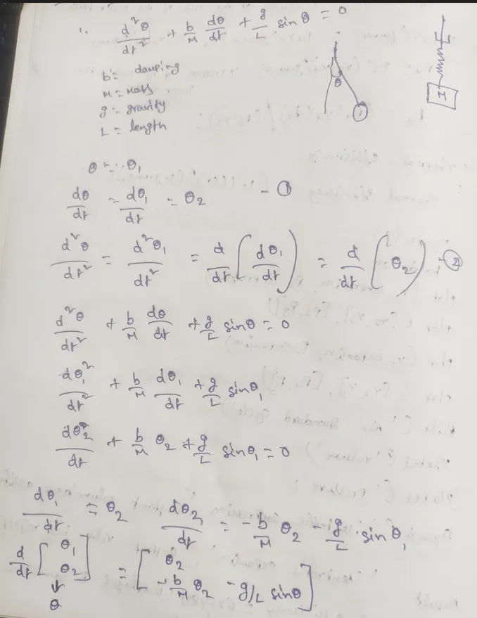
Now we are converting second order ode to first order and the formulas mentioned in the below pic.

Inputs are taken as given in the problem

b =0.05

m = 1kg

l = 1meter

g = 9.81m/s^2

Initial condition are taken as/

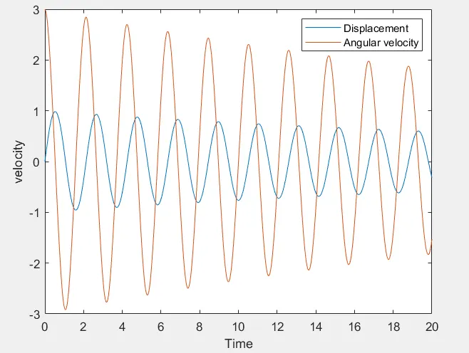
Angular displacement = 0

Angular velocity = 3rad/sec, at time t=0;

the time motion given is between 0-20sec

CODE EXPLANATION:

• First create the function ode
• Initially providing the all inputs like mass of the ball,length of the pendulum,gravity and drag co-efficient
• Providing the angular displacement and angular velocity
• Providing the time span Using linspace command
• Using ode45 command to solve ode equation and call the function of ode
• Plotting the angular displacement and angular velocity graph
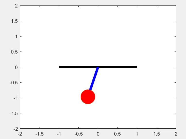
• using for loop command to simulation of the simple pendulum corresponding to the second order ODE
• Fixing the coordinates of the pendulum
• Marker command used for making bob of pendulum
• axis command used to fix the axis
• counter command used to make value changes in each for loop
• movie command used to store all in a single variable
• videoWriter command used to create a videofile.

Ode45_function program:

function[dtheta_dt]= ode_func(t,theta,b,g,l,m)

         theta1 = theta(1)
         theta2 = theta(2)
         dtheta1_dt = theta2;
         dtheta2_dt = -(b/m)*theta2 -(g/l)*sin(theta1);
         dtheta_dt = [dtheta1_dt; dtheta2_dt];

end

Main Program:

close all
clear all
clc

% inputs

b= 0.05;  % Damping coefficient
g = 9.81; % gravity in m/s^2
l=1;     % length of the pendulum in meter
m= 1;   % mass in kgs

% initial condition

theta_0 =[0;3];

% time points

t_span = linspace(0,20,500);

% solve ODE

[t, results] = ode45(@(t,theta)ode_func(t,theta,b,g,l,m),t_span,theta_0);

plot(t,results(:,1))
hold on
plot(t,results(:,2))
ylabel('velocity')
xlabel('Time')
legend('Displacement','Angular velocity')
hold off
% iteration using for loop to create animation of simple pendulum
ct=1;
theta_1 = results(:,1);

for i= 1:length(results(:,1))

     % initial coordinates
     x_start =0;
     y_start =0;
     theta_2 = theta_1(i);

     %final co-ordinates
     x_end = 1*sin(theta_2);
     y_end = -1*cos(theta_2);


     %plotting for animation

     figure(2)
     %base of pendulum
     plot([-1,1],[0,0],'linewidth',4,'color','black')
     hold on
     % string of pendulum
     line([x_start x_end],[y_start y_end],'linewidth',5,'color','b')
     hold on
     %bob of pendulum
     plot(x_end,y_end,'marker','o','MarkerSize',30,'MarkerFaceColor','r')
     axis([-2 2 -2 2])
     pause(0.03)
     hold off
     M(ct)=getframe(gcf);
     ct=ct+1;
end
% creating movie from captured frames
movie(M)
videofile= VideoWriter('simple_pendulum.avi','uncompressed AVI');
open(videofile);
writeVideo(videofile,M);
close(videofile);

ERRORS FACED:

1. Unrecognized function or variable o

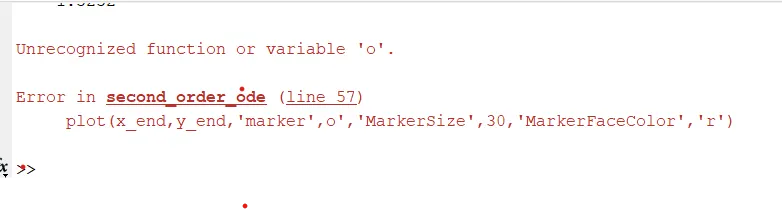
the main issue is typo mistake and we are not given ' before the O.

After correctig like below plot came properly.

RESULT:

• Angular displacement and angular velocity plots were generated for a time range of 20secs

PENDULUM:

CONCLUSION:

We have successfully solved the second order ODE

The animation of the pendulum you tube link is here

https://youtu.be/dG_3TM3N3hg