Week 3 - Solving second order ODEs

Introduction:

The pendulum is a body or mass suspended from a fixed point so that it can swing back & forth under the influence of gravity. Pendulums are regalate the movement of clocks because the interval of time for each complete oscillation, called the period, is constant. The period depends on the length of the pendulum and also to a slight degree on the amplitude, the width of the pendulum's swing.

Aim: 

To solve the 2nd order ODE function using Matlab which depicts the motion of the pendulum & to create an animation of the same.

Objective:

In Engineering, ODE is used to describe the transient behavior of a system. A simple example is a pendulum. The way the pendulum moves depends on the Newtons second law. When this law is written down, we get a second order Ordinary Differential Equation that describes the position of the "ball" w.r.t time.  Similarly, there are hundreds of ODEs that describe key phenomena and if you have the ability to solve these equations then you will be able to simulate any of theses systems.

To write a program that solves the following ODE. This ODE represents the equation of motion of a simple pendulum with damping

In the above equation,

g = gravity in m/s2,

L = length of the pendulum in m,

m = mass of the ball in kg,

b=damping coefficient.

Fixed Parameters:

L=1 metre.

m=1 kg.

b=0.05.

g=9.81 m/s2.

time period= 0-20 sec.

angular displacement=0.

angular velocity=3 rad/sec at time t=0.

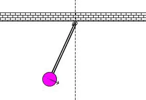
When you do this you will get the position of the pendulum as a function of time. Use this information to animate the motion of the pendulum, as shown in the below figure.

                                   

Main Program:

% To Simulate the transient behaviour of a Simple pendulum

clear all
close all
clc

% Inputs
b = 0.05;  % damping co.efficient
g = 9.81;  % gravity
l = 1;    % length of the pendulum
m = 1;  % mass 

% Initial condition
theta_0 = [0;3];  

% Time points
t_span = linspace(0,20,200);

% Solving ODE

[t, results] = ode45(@(t, theta)ode_45_function(t, theta, b, g, l, m), t_span, theta_0);

plot(t, results(:,1))
hold on 
plot(t, results(:,2))
ylabel('Velocity(Red) & Displacement(Blue)')  % name of Y axis
xlabel('Time')     % name of X axis
title('Simple Pendulum with damping (ODE Function)')    % gives title to the plot

% Iterations using for loop to create animation of simple pendulum

ct = 1;   % initiate the counter value
theta_1 = results(:,1);

for i = 1:length(results(:,1))

    % Initial Co-ordinates
    x0 = 0;
    y0 = 0;
    theta_2 = theta_1(i);

    % Final Co-ordinates
    x1 = l*sin(theta_2);
    y1 = -l*cos(theta_2);

    % Plotting for animation
    figure(2)
    plot([-1 1],[0 0],'LineWidth',4,'Color','b')   % Base of Pendulum
    hold on
    plot([x0 x1],[y0 y1],'linewidth',4,'Color','g','Marker','o','MarkerSize',15,'MarkerFaceColor','r')   % String & Bob of pendulum
    axis([-2 2 -2 2])
    pause(0.03)
    hold off
    M(ct) = getframe(gcf);
    ct = ct + 1;
end
   
% Movie & Videofile
movie(M)
v_f = VideoWriter('Pendulum Challenge.avi','Uncompressed AVI');
open(v_f)
writeVideo(v_f,M)
close(v_f)

Function Program:

function [dtheta_dt] = ode_45_function(t, theta, b, g, l, m)

theta1 = theta(1);
theta2 = theta(2);
dtheta1_dt = theta2;
dtheta2_dt = -(b/m)*theta2 - (g/l)*sin(theta1);
dtheta_dt = [dtheta1_dt; dtheta2_dt];

end

Stepwise Explanation:

• In step one, input & initial condition of a simple pendulum are fed.
• Then the program is written to solve the ODE in which Matlab inbuilt function (ode45) is used with constant theta, t, and another function is used which is defined separately in function program.
• In the next step result of solved ODE is plotted with respect to time using plot command.
• Iteration of co-ordinate is now fed using for loop to create animation.
• Then plot command is used to plot pendulum string and bob.
• In the next step, the move command is used to create an animated video of oscillating pendulum.

Explanation:

• In the above program, the fixed parameters are length, mass, damping coefficient, and acceleration due to gravity.
• Time and angle are given as the initial condition.
• In the tspan command, 200 values are taken in between 0 to 20 times period.
• Using the ode45 command ODE function is introduced.
• Using the plot command velocity & displacement is plotted in the Y axis against time in the X axis.
• Using the for loop command the mass at various points & various times are marked in the graph and are plotted.
• Using the movie command the plot is saved as an uncompressed avi file.

Conclusion:

The simulation of the transient behaviour of a simple pendulum is successfully created by using a program in Matlab.

Animation Link:

https://drive.google.com/file/d/1Zik53UEjdO-f3BjVuxGGh8xFwZfyxz_8/view?usp=sharing