CURVE FITTING

Aim:

To perform a curve fitting for the given dataset, to show splitwise method & to find the best fit & perfect fit for that particular dataset using Matlab.

Objective:

• Write code to fit a linear & cubic polynomial for the Cp data.
• Plot the linear & cubic fit curves along with the raw data points. Title & axes labels are a must, legends could be shown if neccessary.
• Explain the parameters used to measure the fitness characteristics for both the curves.

Curve Fitting:

1. Curve fitting is the process of constructing a curve or mathematical function, that has the best fit to a series of data points, possibly subjected to constraints.
2. Curve fitting can involve either interpolation, where an exact fit to the data is required, or something, in which a "smooth" function is constructed that approximately fits the data.
3. Fitted curves can be used as an aid for data visualization, to infer values of a function where no data are available, & to summarize the relationship among two or more variables.

Fitting a Curve:

• The first-degree polynomial equation: Y = ax + bis a line with slope a. A line will connect any two points, so a first degree polynomial equation is an exact fit through any two points with distinct X co-ordinates.
• If the order of the equation is increased by to a second-degree polynomial the following equation is obtained: Y = ax^2 + bx + c. This will exactly fit a simple curve to three points.
• If the order of the equation is increased to a third-degree polynomial, Y = ax^3 + bx^2 + cx + d. This will exactly fit four points.

Parameters used to measure the fitness of the curve:

The parametric models used to measure the fitness of the curve:

• Sum of Squares due to Errors: This statistics measures the total deviation of the response values from the fit to the response values. It is also called the summed square of residuals and is usually labelled as SSE. A value closer to 0 indicates a better fit.

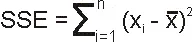
• R-Square: This statistics measures how successful the fit is in explaining the variation of the data. Put another way, R-Square is the square of the correlation between the response values and the predicted response values. It is also called the square of the multiple correlation coefficient and the coefficient of multiple determination. R-Square is defined as the ratio of the sum of squares of the regression (SSR) and the total sum of squares(SST).

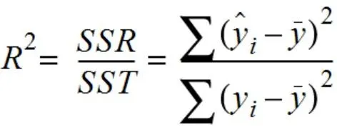
SST = SSR + SSE

R-Square can take on any value between 0 & 1, with a value closer to 1 indicating a better fit.

• Degrees of Freedom Adjusted R-Square: This statistics uses the R-Square statistics defined above, and adjusts it based on the residual degrees of freedom is defined as the number of response values n minus the number of fitted coefficients m estimated from the response values. The adjusted R-Square statistics can take on any value less than or equal to 1, with a value closer to 1 indicating a better fit.
• Root Mean Squared Error: This statistics is also known as the fit standard error & the standard error of the regression. An RMSE value closer to 0 indicates a better fit.

Program:

Linear Fit:

clear all
close all
clc

% Loading the data to matlab
cp_data = load('data');
temperature = cp_data(: , 1);  % First column is temperature data
cp = cp_data(: , 2);  % Second column is Cp data

% Curve fit
% Considering first order polynmial 
% cp = a*T + b*T
co_effs = polyfit(temperature, cp, 1);    % polyfit command to estimate coefficients i.e. a,b
predicted_cp = polyval(co_effs, temperature);     % polyval to calculate predicted value of Cp

% Compare curve fit with the original data
plot(temperature, cp, 'linewidth', 3,'Color','b')   % plotting cuvre to original observed data
hold on 
plot(temperature, predicted_cp,'linewidth',3,'Color','r')   % plotting curve to predicted data
xlabel('Temperature [K]')    % labelling X-axis as Temperature
ylabel('Specific Heat [KJ/Kmol-K]')     % labelling Y-axis as Cp
axis([0 4000 900 1400])   % defining axis limits
legend('Original dataset','Curve fit')  % providing legends to curves

Cubic Fit:

clear all
close all
clc

% Loading the data to matlab
cp_data = load('data');
temperature = cp_data(: , 1);  % First column is temperature data
cp = cp_data(: , 2);  % Second column is Cp data

% Curve fit
% Considering cubic polynmial 
% cp = a*T^3 + b*T^2 + c*T + d
co_effs = polyfit(temperature, cp, 3);    % polyfit command to estimate coefficients i.e. a,b
predicted_cp = polyval(co_effs, temperature);     % polyval to calculate predicted value of Cp

% Compare curve fit with the original data
plot(temperature, cp, 'linewidth', 3,'Color','b')   % plotting cuvre to original observed data
hold on 
plot(temperature, predicted_cp,'linewidth',3,'Color','r')   % plotting curve to predicted data
xlabel('Temperature [K]')    % labelling X-axis as Temperature
ylabel('Specific Heat [KJ/Kmol-K]')     % labelling Y-axis as Cp
axis([0 4000 900 1400])   % defining axis limits
legend('Original dataset','Curve fit')  % providing legends to curves

Steps Taken:

• Start the program with 'clear all','close all',and 'clc' commands.
• The data of specific heat is loaded with 'load' command and 'Temperature', as well as 'Cp' array, is defined.
• Curve fitting is performed using 2 funtions:
• (i)Polyfit is a Matlab function that computes a least-squares polynomial, which can be used to model a curve to fit the data.
• (ii) Polyval evaluates a polynomial for a given set of x values. So Polyval generates a curve to fit the data based on the coefficients found using polyfit.
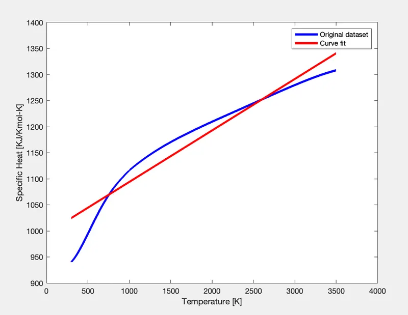
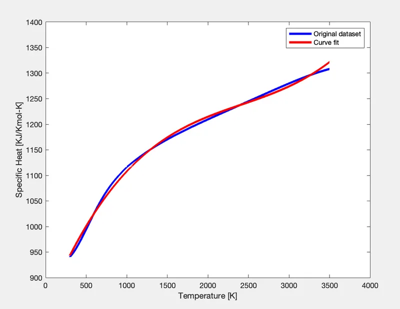
• The curve fit data is compared with original data by plotting the curves to get linear and cubic curve fitting.
• The axis is shifted by using the 'axis' command and the legend is provided for the plot.

BEST FIT:

• It means that the differences between the actual measured values & the values predicted by the model equation minimized.

PERFECT FIT:

• When the curve goes through every point the sum-of-squares is 0, & the R2 is 100.

HOW TO GET THE BEST FIT?

• The degrees of the polynomial affects the 'detail' to which it approximates your data.
• At first-degree polynomial is a Simple linear fit: Y = a(1)X + b(2), the degree being one less than the no. of parameters of thw polynomial estimates. The higher the polynomial degrees, the more closely the polynomial fits the data. Lower degrees have the effect of 'smoothing' the fit, acting as a sort of lowpass filter. The hightest possible degree is one less than the no. of data points to be fit, although a polynomial degree higher than about 7 does not add any significant information. Choosing the polynomial degree ( as with most other aspects of signal processing) is a matter of experimenting to determine what works best.
• To see the effect polynomial degree, the easiest way is to experiment with the core MATLAB functions polyfit & polyval with random data (the third argument to polyfit is the polynomial degree).
• The third-degree polynomial approximates the sine curve. Note that the 9-degree polynomial fits the data more closely, but does not at all approximate the sine curve (and also throws an error).

Improved Cubic Fit:

clear all
close all
clc

% Loading the data to Matlab
cp_data = load('data');
temperature = cp_data(: , 1);
cp = cp_data(: , 2);

% Splitting data
temperature1 = cp_data(1:800,1);
cp1 = cp_data(1:800,2);

temperature2 = cp_data(801:1600,1);
cp2 = cp_data(801:1600,2);

temperature3 = cp_data(1601:2400,1);
cp3 = cp_data(1601:2400,2);

temperature4 = cp_data(2401:3200,1);
cp4 = cp_data(2401:3200,2);


% Considering Cubic polynomial | Y = aX + b
co_eff1 = polyfit(temperature1,cp1,3);
pred_cp1 = polyval(co_eff1,temperature1);

co_eff2 = polyfit(temperature2,cp2,3);
pred_cp2 = polyval(co_eff2,temperature2);

co_eff3 = polyfit(temperature3,cp3,3);
pred_cp3 = polyval(co_eff3,temperature3);

co_eff4 = polyfit(temperature4,cp4,3);
pred_cp4 = polyval(co_eff4,temperature4);

% Plotting Results
plot(temperature,cp,'LineWidth',3,'Color','b')
hold on
plot(temperature1,pred_cp1,'LineWidth',3,'Color','r')
hold on
plot(temperature2,pred_cp2,'LineWidth',3,'Color','r')
hold on
plot(temperature3,pred_cp3,'LineWidth',3,'Color','r')
hold on
plot(temperature4,pred_cp4,'LineWidth',3,'Color','r')
hold on
xlabel('Temperature [K]')    % labelling X-axis as Temperature
ylabel('Specific Heat [KJ/Kmol-K]')     % labelling Y-axis as Cp
axis([0 4000 900 1400])   % defining axis limits
legend('Original dataset','Curve fit')  % providing legends to curves

Result:

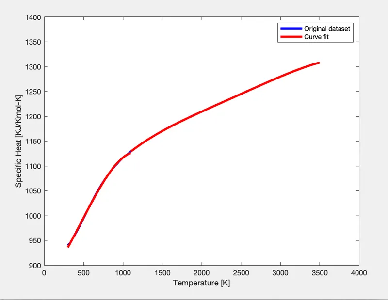
Conclusion:

1. By splitting the data we get a better fit, more the no. of splits, the better is the output results.
2. There are many methods that can be used to make the curve fit properly.
3. We need to have high order polynomial equatiobs to achieve the best fit.

References:

• https://skill-lync.com/student-projects/Curve-Fitting-and-criterion-to-choose-best-fit-41860
• https://en.wikipedia.org/wiki/Curve_fitting
• https://in.mathworks.com/help/curvefit/curve-fitting.html