Week 3 - Solving second order ODEs

Aim:

To solve the ODE which represents the equation of motion of a simple pendulum with damping.

Objectve:

• To create the program to solve the second-order equation represents the equation of motion of a simple pendulum with damping
• To create an animation video of output by obtained by solving the ODE.

Theory:

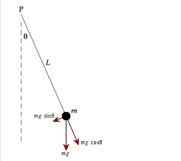
The motion of a simple pendulum is a basic classical example of simple harmonic motion,consisting of a small bob and a massless string. Movement of pendulum depends on Newton second law. Differential equation is formed by position of the end of the pendulum with respect to time.

simple pendulum with FBD

The equation of motion is

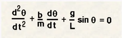
In the above equation is

g = gravity in m/s^2.

L = length of the pendulum in metre.

m = mass of the ball in kg.

b = damping coefficient.

since it is second-order equation we will convert it to first order equation to solve using ode45 solver in MATLAB.

Let

`theta = theta1`

`(d theta1)/dt = theta2`

`(d theta^2)/(dt)^2 = (d theta2)/dt`

Input

• l = 1metre.
• m = 1 kg
• b = 0.05
• g = 9.81 m/s^2.
• Time span = 0-20 sec.
• Angular displacement = 0
• Angular Velocity = 3rad/sec^2 at t=0.

Code for Function Program.

function [dtheta_dt] = ode_function(t,theta,b,g,l,m)

theta1 = theta(1);
theta2 = theta(2);
dtheta1_dt = theta2;
dtheta2_dt = -(b/m)*theta2 - (g/l)*sin(theta1);
dtheta_dt = [dtheta1_dt;dtheta2_dt];

end

Final Program:

clear all
close all
clc

% Input data
l = 1; % meter
m = 1; % kg
b = 0.05;
g = 9.81; % m/sec^2

% time span for pendulum
t_span = linspace(0,20,500);

% Initial condition
theta_0 = [0;3];  % 1st column represent displacement & 2nd column represent velocity

% solving ode by ode45
[t,results] = ode45(@(t,theta) ode_function(t,theta,b,g,l,m),t_span,theta_0);

% plotting for analysing pendulum transition behaviour
figure(1)
plot(t,results(:,1)) %plotting graph for time vs results(:,1) which is displacement
hold on
plot(t,results(:,2)) % plotting graph for time vs results(:,2) which is velocity
xlabel('Time')
ylabel('Displacement/Velocity')
legend('displacement','velocity')
grid on
hold off

loop_counter = 1

for i = 1:length(results(:,1)) % assign the value of i

% Starting point of pendulum which is fixed

x0 = 0;
y0 = 0;

% varied value of end point of pendulum
x1 = l*sin(results(i,1));
y1 = -l*cos(results(i,1));

figure(2)

plot ([-1 1],[0 0],'linewidth',8) % plotting fixed point of the roof

hold on
plot([x0 x1],[y0 y1],'linewidth',3) 

plot(x1,y1,'marker','O','markersize',30,'MarkerFaceColor','b')

plot(x0,y0,'marker','O','markerSize',9,'MarkerFaceColor','y')

plot([x0 x0],[y0 -1.5],'LineStyle','--','Color','r','LineWidth',3)

grid on

axis('tight')

hold off

pause(0.0000003)

M(loop_counter) = getframe(gcf)
 loop_counter = loop_counter + 1  
end

movie(M)
videofile = VideoWriter('pendulum_movement.mp4','Uncompressed AVI');
open(videofile)
writeVideo(videofile,M)
close(videofile)

Program Explanation:

In the first step input & initial conditions is fed-in MatLab.

[t,results] = ode45(@(t,theta) ode_function(t,theta,b,g,l,m),t_span,theta_0);

The program is written to solve the ODE in which MATLAB is inbuilt function (ode45) is used with constant theta,t, and another function.

figure(1)

plot(t,results(:,1)) %plotting graph for time vs results(:,1) which is displacement

hold on

plot(t,results(:,2)) % plotting graph for time vs results(:,2) which is velocity

xlabel('Time')

ylabel('Displacement/Velocity')

legend('displacement','velocity')

grid on

hold off

This result of ODE is plotted with respect to time using plot command.

loop_counter = 1

for i = 1:length(results(:,1)) % assign the value of i

next to create animation we used Loop command.

we used displacement values result(:,1).

% Starting point of pendulum which is fixed

x0 = 0;

y0 = 0;

% varied value of end point of pendulum

x1 = l*sin(results(i,1));

y1 = -l*cos(results(i,1));

to find x1 & y1 we use result(i,1) because we need to substitute all value in 1st column.

figure(2)

plot ([-1 1],[0 0],'linewidth',8) % plotting fixed point of the roof

hold on

plot([x0 x1],[y0 y1],'linewidth',3)

plot(x1,y1,'marker','O','markersize',30,'MarkerFaceColor','b')

plot(x0,y0,'marker','O','markerSize',9,'MarkerFaceColor','y')

plot([x0 x0],[y0 -1.5],'LineStyle','--','Color','r','LineWidth',3)

grid on

axis('tight')

hold off

plotting all values in chart using the plot command.
axis('tight') is used to adjust the graph to correct size without manual entry.

pause(0.0000003)

M(loop_counter) = getframe(gcf)

loop_counter = loop_counter + 1

end

pause to stop at each loop ends.
M(loop_counter) which collects all 500 plot data in picture format in sequence order mentioned in program.

movie(M)

videofile = VideoWriter('pendulum_movement.mp4','Uncompressed AVI');

open(videofile)

writeVideo(videofile,M)

close(videofile)

Using M movie command converts the collection of pictures into video format.

OUTPUT:

The output obtained is a graphical representation of the velocity curve & displacement curve with respect to time.

The output obtained is an Animation video of output obtained by solving the ODE with respect to time & displacement
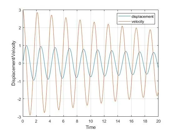
the video is uploaded on youtube.

https://youtu.be/Nm4KHXfSW98

Error faced during Programing:

spelling mistake in the written function

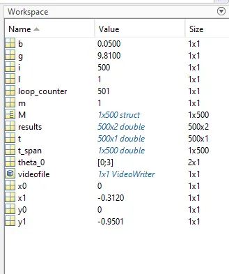
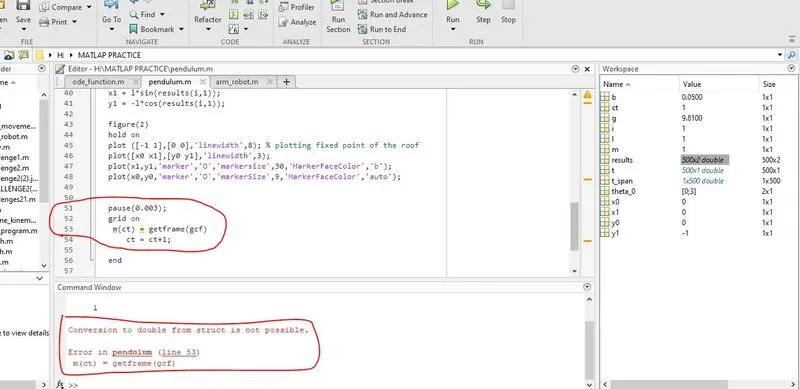
The Error is due to the 53 line m

the same small letter m is used in the mass value of Bob in pendulum. latter I used Capital letter M in storing the pictures.

I used hold on in 44 line so that it shows the all 500 oscillation values by overlapping in the chart.

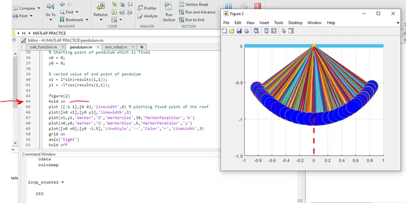
Then later I changed the hold on before plot([x0 x1],[y0 y1],'linewidth',3) so that the problem is Resolved.

Conclusion:

The simulation of the transient behaviour of a simple pendulum is successfully created by using program in MATLAB.