Week 3 - Solving second order ODEs

Course: MATLAB for Mechanical Engineers

Challenge: Solving Second-Order ODEs

Submitted By: Amanpreet Singh Whan

1 Aim:

The aim of the week 3 challenge is to write a program in MATLAB to solve second-order Ordinary Differential Equation (ode).

2 Theory and Governing Equations:

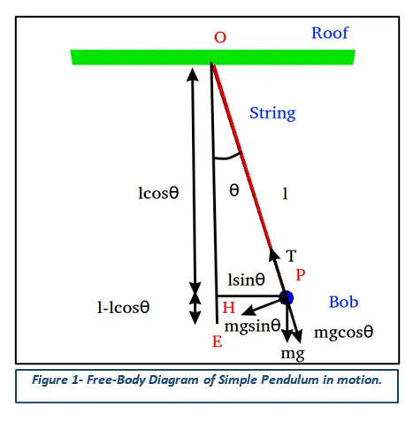
The simple pendulum is another mechanical system that moves in an oscillatory motion. It consists of a point mass ‘m’ suspended by means of a light inextensible string of length L from fixed support as shown in Fig 1. The motion occurs in a vertical plane and is driven by a gravitational force. The forces which are acting on the mass are shown in the figure. The tangential component of the gravitational force, mg sin θ, always acts towards the mean position θ = 0 opposite to the displacement, restoring force acting tangent to the arc.

In Engineering, ODE is used to describe the transient behavior of a system. A simple example is a pendulum. The way the pendulum moves depends on Newton’s second law. This law derives a second-order Ordinary Differential Equation that describes the position of the ball of the pendulum w.r.t time.

Simple Pendulum

The free-body diagram of a simple pendulum in motion is represented by the following figure1.

L = 1 m is the length of the pendulum.

m = 1 kg is the mass of the ball.

b = 0.05 is the damping coefficient.

g = 9.81 m/s^2 is the gravity.

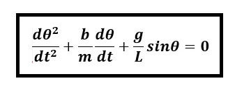
The ODE that represents the equation of motion of a simple pendulum with damping is as follows:

3 Objectives:

The objectives of the week 3 challenges are as follows:

• Write a program that can solve 2^nd order ODE and simulate the simple motion of the pendulum for 20 seconds.
• Create an animation file for the obtained results using the “Image Magick” software for the same.

4 Body of the Content:

MATLAB (an abbreviation of "MATrix LABoratory") is a proprietary multi-paradigm programming language and numeric computing environment developed by MathWorks. MATLAB allows matrix manipulations, plotting of functions and data, implementation of algorithms, creation of user interfaces, and interfacing with programs written in other languages. Although MATLAB is intended primarily for numeric computing, an optional toolbox uses the MuPAD symbolic engine allowing access to symbolic computing abilities. An additional package, Simulink, adds graphical multi-domain simulation and model-based design for dynamic and embedded systems.

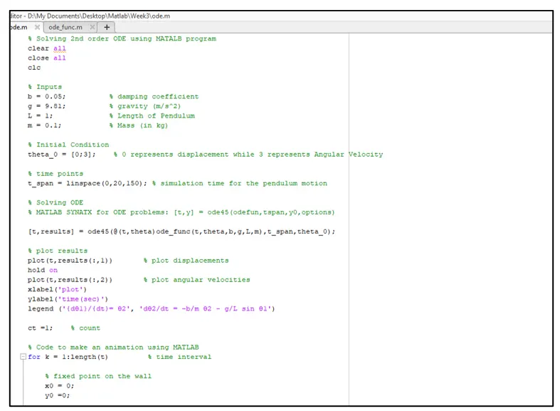
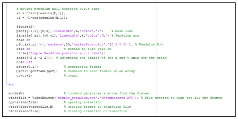
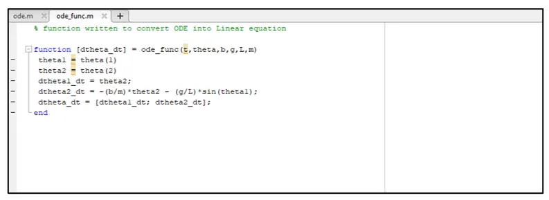
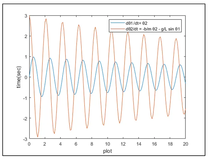
The code was written to fulfill the requirements of the Week 3 challenge and is attached in the following figures. In addition, the animation created from the plots obtained from the written code is attached as well.

Youtube Link for the Simple Pendulum Animation:

https://youtu.be/hspbkAw1Vw8

5 Conclusion:

In conclusion, the main aim of the week 3 challenge is to write a MATLAB program to solve second-order Ordinary Differential Equation. In addition, create an animation file to simulate the motion of a simple pendulum.

6 Appendix:

% Solving 2nd order ODE using MATALB program
clear all
close all
clc

% Inputs
b = 0.05;          % damping coefficient
g = 9.81;          % gravity (m/s^2)
L = 1;             % Length of Pendulum
m = 1;           % Mass (in kg)

% Initial Condition
theta_0 = [0;3];    % 0 represents displacement while 3 represents Angular Velocity

% time points 
t_span = linspace(0,20,150); % simulation time for the pendulum motion

% Solving ODE
% MATLAB SYNATX for ODE problems: [t,y] = ode45(odefun,tspan,y0,options)

[t,results] = ode45(@(t,theta)ode_func(t,theta,b,g,L,m),t_span,theta_0);

% plot results
plot(t,results(:,1))       % plot displacements
hold on
plot(t,results(:,2))       % plot angular velocities
xlabel('plot')
ylabel('time(sec)')
legend ('{dθ1}/{dt}= θ2', 'dθ2/dt = -b/m θ2 - g/L sin θ1')

ct =1;    % count

% Code to make an animation using MATLAB
for k = 1:length(t)         % time interval
    
    % fixed point on the wall
    x0 = 0;
    y0 =0;
    
    % moving pendulum ball position w.r.t time
    x1 = L*sin(results(k,1));
    y1 = -L*cos(results(k,1));
    
    figure(2)
    plot([-1,1],[0,0],'linewidth',6,'color','r')    % base line
    line([x0 x1],[y0 y1],'linewidth',4,'color','b') % Pendulum arm 
    hold on
    plot(x1,y1,'o','markers',20,'markerfacecolor','[0.2 0 0]'); % Pendulum Bob
    grid on                 % comand to turn grid on
    title('Simple Pendulum position w.r.t time');
    axis([-2 2 -2 2]);  % adjusting the limits of the x and y axis for the graph
    hold off
    pause(0.1);             % generating frames
    M(ct)= getframe(gcf);   % command to save frames in an array
    ct=ct+1;                % count

end

movie(M)                    % command generates a movie from the frames
videofile = VideoWriter('simple_pendulum.avi','Uncompressed AVI'); % file created to dump out all the frames
open(videofile)             % opening animation
writeVideo(videofile,M)     % writing frames to animation file
close(videofile)            % closing animation or videofile

% function written to convert ODE into Linear equation

function [dtheta_dt] = ode_func(t,theta,b,g,L,m)
 theta1 = theta(1)
 theta2 = theta(2)
 dtheta1_dt = theta2;
 dtheta2_dt = -(b/m)*theta2 - (g/L)*sin(theta1);
 dtheta_dt = [dtheta1_dt; dtheta2_dt];
end