Week 3 - Solving second order ODEs

https://youtu.be/3KHWhQZe8r8

SECOND ODE OF PENDULUM

Aim: Solve second order differential equation for an oscillating pendulum using MATLAB

Objectives: 1) Generate a MATLAB code for an oscillating pendulum

2) Working animation of pendulum using ode45 built-in function.

Theory:

A simple pendulum is a mechanical system which consists of a light inextensible string and a small bob of some mass which is made to oscillate about its mean position from left extreme to right extreme.

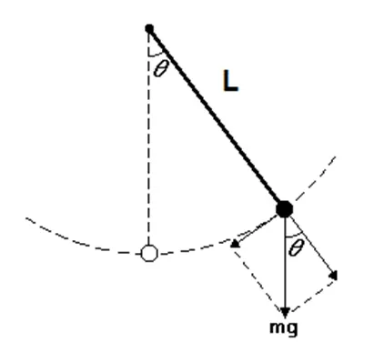
the second-order equation describing the motion of a pendulum is,

`d^2Ө/(dt^2 )=-(b/m) dӨ/dt-(g/L)sinӨ`

Here Ө is the angle the pendulum has moved from the vertical, L is the length of the pendulum, g is the acceleration due to gravity, m is the mass of the pendulum, and b is a damping coefficient. See the figure above,

Mathematical Calculations:

The expression for second ODE for oscillating pendulum is,

`(d^2 Ө)/(dt^2 )=-(b/m) dӨ/dt-(g/L)sinӨ`

Or,

`(d^2 Ө)/(dt^2 )+(b/m) dӨ/dt+(g/L)sinӨ=0`

Consider, Ө=Ө₁ then,

`dӨ/dt=dӨ_1dt=Ө2--------------(1)`

`(d^2 Ө)/(d^2 t)=(d^2 Ө_1)/(d^2 t)=d/dt ((dӨ_1)/dt)=(dӨ_2)/dt--------------(2)`

Where ,

`Ө_2=(dӨ_1)/dt`

We have,

`(d^2 Ө)/(dt^2 )+(b/m) dӨ/dt+(g/L)sinӨ=0`

`(d^2 Ө_1)/(dt^2 )+(b/m) (dӨ_1)/dt+(g/L)sinӨ_1=0`

`(dӨ_2)/dt+(b/m) Ө_2+(g/L)sinӨ_1=0`

`(dӨ_2)/dt=-(b/m) Ө_2-(g/L)sinӨ_1--------------(3)`

Matrix,

`d/dt [Ө_1 ;Ө_2 ]=[Ө_2;-(b/m) Ө_2-(g/L)sinӨ_1 ]`

CODE or The program:

%The function code

%The matrix is solved

• function[dtheta_dt]=ode_pend(t,theta,b,g,L,m)
• theta1=theta(1)
• theta2=theta(2)
• dtheta1_dt=theta2;
• dtheta2_dt=-(b/m)*theta2-(g/L)*sin(theta1);
• dtheta_dt=[dtheta1_dt;dtheta2_dt];

%main program

• clear all
• close all
• clc

%inputs

• L=1; %length of the string
• m=1; %mass of bob
• g=9.81; %acceleration due to gravity
• b=0.05; %damping coefficient
• ct=1; %counter

%initial conditions

• dis_vel=[0;3]; %Displacement is 0, Angular velocity is 3rad/sec
• t_span=linspace(0,20,500); %Timmer

%ODE function calling

%ode45 is a built-in function called ODE solver

• [t,result]=ode45(@(t,theta) ode_pend(t,theta,b,g,L,m),t_span,dis_vel);

• figure(1)
• hold on

• plot(t,result(:,1),'color','r') %plots Angular Displacement
• plot(t,result(:,2),'color','b') %plots Angular Velocity
• xlabel('Time in sec')
• ylabel('Angular displacement in rad & Angular Velocity in rad/sec')
• grid on
• title('Simple Pendulum','Color','r')
• legend('Angular displacement','Angular velocity')

%input for pendulum oscillation

• amplitude=result(:,1);
• for i=1:length(amplitude);
• angle=amplitude(i);
• x0=0;
• y0=0;

• x1=L*sin(angle);
• y1=-L*cos(angle);

%plotting the pendulum

• figure(2)
• plot([-0.5 0.5],[0 0],'color','b','LineWidth',5) %base line or reference
• hold on
• plot([x0 x1],[y0 y1],'Color','r','LineWidth',2) %string

• plot(x1,y1,'Marker','O','MarkerFaceColor','y') %Bob or weight
• hold off

• grid on
• axis([-1.5 1.5 -1.5 0.5]); %pendulum fit area
• pause(0.005)

%creating animation video of pendulum

• M(ct)=getframe(gcf);
• ct=ct+1

• end
• movie(M)
• videofile=VideoWriter('second_ODE_pendulum.m','Uncompressed AVI')
• open(videofile)
• writeVideo(videofile,M)
• close(videofile)

Observations:

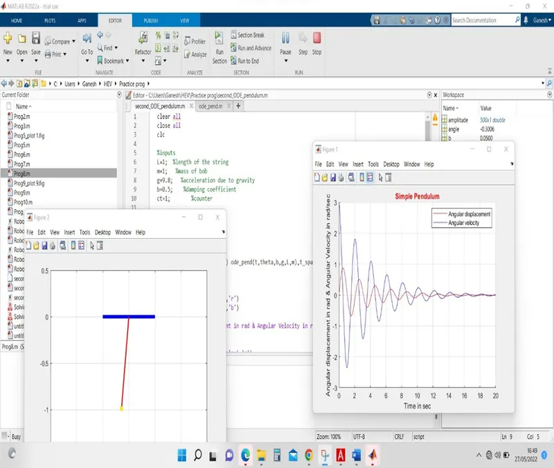
• The plot with higher damping coefficient, b=0.5

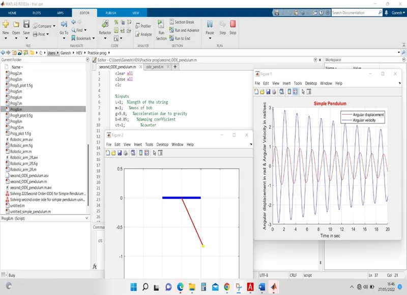
• The plot with damping coefficient, b=0.05

Conclusions:

• Simulation of simple pendulum is done using ode45 command.
• The influence of damping coefficient is verified.
• The video of simple pendulum has been uploaded on youtube. Follow the link: https://youtu.be/3KHWhQZe8r8