Air Standard Otto Cycle with thermal efficiency using MATLAB
AIR STANDARD OTTO CYCLE
Aim: To create working principle of Air Standard Otto Cycle using MATLAB.
Objectives: 1) Generate code to plot PV-diagram for Otto Cycle.
2) Calculate thermal efficiency for Otto Cycle.
Theory:
The Otto cycle is one of the reference cycles for IC engines. It is also called as constant volume heat addition cycle. This cycle is Isentropic, adiabatic and reversible process.
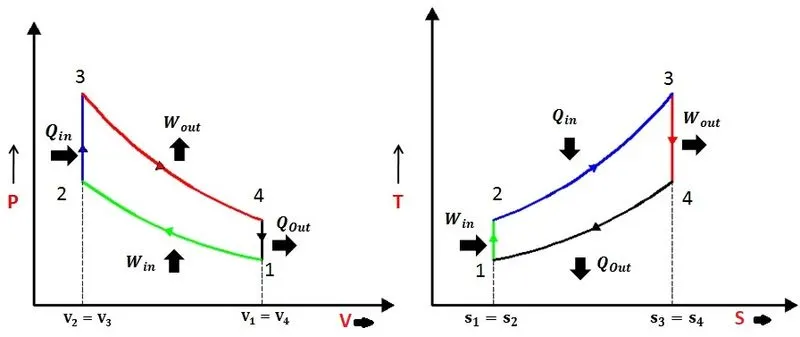
The plot below gives P-V and T-S diagrams for Otto cycle,
The stages in the Otto cycle are,
- Reversible adiabatic (Isentropic) compression - 1 to 2
- Constant volume heat addition - 2 to 3
- Reversible adiabatic (Isentropic) expansion - 3 to 4
- Constant volume heat rejection - 4 to 1
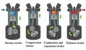
The Otto cycle for sparkplug ignition (SI) engine works under 4-stroke design will rotate the crank shaft by 2 complete revolutions. In the analysis the suction and exhaust are neglected.
Mathematical Calculations:
- Swept Volume (Vs) is given by,
`Vs=(πd^2)/4 L`
Where d is diameter of the cylinder, L is stroke length
- Clearance Volume (Vc),
`Vc=(Vs)/(c_r-1)`
Where cr is compression ratio
- `PV^γ=constant`
Where P is Pressure of the system, V is volume of the system, is called gamma, the gas ratio
- `(PV)/T=constant`
Where T is temperature
- `V/(Vc)=1+1/2 (c_r-1)[R+1-cosӨ-(R^2-sin^2 Ө)^(1/2)]`
where V is volume of the system at angle Ө, R is Ratio of length of connecting rod (l) to crank pin radius (a), cr is compression ratio
Also, crank pin radius (a) = stroke length (L)/2
CODE or The program:
- clear all
- close all
- clc
%inputs
- gamma=1.4
- t3=2300
- p1=101325 %state variables
- t1=500
- bore=0.1; %engine geometricparameters
- stroke=0.1;
- con_rod=0.15;
- cr=12;
%calculating the swept volume and the clearance volume
%swept volume is the theorical volume considering the respective dimensions
%clearance volume is the unusable space ex: left-out diameter or stroke length during working.
% The air that is sucked into cylinder during suction stroke undergoes reversible adiabatic (isentropic) compression. Since the air is compressed, the pressure increases from P1 to P2, the volume decreases from V1 to V2, temperature rises from T1 to T2
- v_swept=(pi/4)*bore^2*stroke;
- v_clearance=v_swept/(cr-1);
- v1=v_swept+v_clearance
- v2=v_clearance
%state variable at state point 2
% This process is an isochoric process i.e. the heat is added to the air at constant volume. Due to the heat addition, the pressure increases from P2 to P3, pressure, volume remains constant(i.e. V2=V3), temperature increases from T2 to T3
% p2v2^gamma=p1v1^gamma
%p2=p1*(v1/v2)^gamma=p1*cr^gamma
- p2=p1*cr^gamma;
%p1v1/t1=p2v2/t2|t2=p2*v2*t1/(p1*v1)
- t2=p2*v2*t1/(p1*v1);
- constant_c=p1*v1^gamma;
- V_compression=engine_kinematics(bore, stroke, con_rod, cr,180,0)
- P_compression=constant_c./V_compression.^gamma
%state variable at state point 3
%The process is isentropic (reversible adiabatic) expansion of air takes place. Here the process involves expansion of air, so the pressure decreases from P3 to P4, volume increases from V3 to V4, temperature falls from T3 to T4
- v3=v2
%p3v3/t3=p2v2/t2|p3=p2*t3/t2
- p3=p2*t3/t2
- constant_c=p3*v3^gamma;
- V_expansion=engine_kinematics(bore, stroke, con_rod, cr,0,180)
- P_expansion=constant_c./V_expansion.^gamma
%state variable at state point 4
%The pressure decreases from P4 to P1, Volume remains constant (i.e. V4=V1), temperature falls from T4 to T1.
- v4=v1
%p3v3^gamma=p4v4^gamma|p4=p3(v3/v4)^gamma
- p4=p3*(v3/v4)^gamma
% thermal efficiency in percentage
- Thermal_Efficiency = (1-(cr^(gamma-1))^-1)*100
% Plotting
- figure(1)
- hold on
- plot(v1,p1,'*','Color','r')
- plot(V_compression,P_compression,'b')
- plot(v2,p2,'*','Color','r')
- plot(v3,p3,'*','Color','r')
- plot(V_expansion,P_expansion,'b')
- plot(v4,p4,'*','Color','r')
- plot([v2 v3],[p2 p3],'Color','g')
- plot([v4 v1],[p4 p1],'Color','g')
- xlabel('Volume (m^3)')
- ylabel('Pressure (KPa)')
Function codes:
function [v]=engine_kinematics(bore, stroke, con_rod, cr, start_crank, end_crank)
a=stroke/2;
R=con_rod/a;
v_s=pi/4*bore^2*stroke;
v_c=v_s/(cr-1);
theta=linspace(start_crank,end_crank,100);
%the total volume of the system formula is converted as below for ease of coding
term1=0.5*(cr-1);
term2=R+1-cosd(theta);
term3=(R^2-sind(theta).^2).^0.5;
v=(1+term1*(term2-term3)).*v_c;
end
Error fixation or fine tuning of codes:
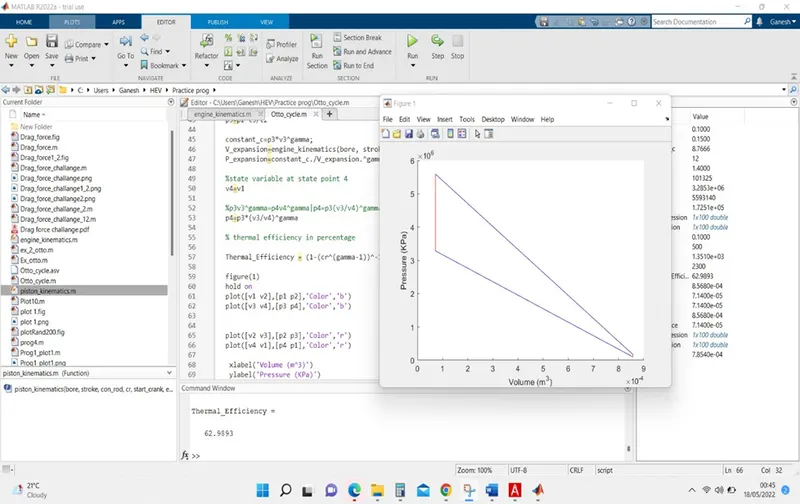
- Assuming the curves are slope i.e., consistently increasing or decreasing but against Otto cycle.. the plot is as below
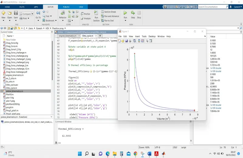
- Considering the variation of volume due to temperature and piston kinematics the slope is defined as a function. The plot is as below also Thermal efficiency on command window
Conclusions:
- The PV-diagram is plotted for Air Standard Otto Cycle using MATLAB.
- Thermal efficiency in percentage is calculated and displayed in command window.
- A separate function code is used to get smooth curve for the cycles.
%Main program code,

clear all
close all
clc

%inputs
gamma=1.4
t3=2300

%state variables
p1=101325
t1=500
%engine geometricparameters
bore=0.1;
stroke=0.1;
con_rod=0.15;
cr=12;

%calculating the swept volume and the clearance volume
v_swept=(pi/4)*bore^2*stroke;
v_clearance=v_swept/(cr-1);

v1=v_swept+v_clearance
v2=v_clearance

%state variable at state point 2
% p2v2^gamma=p1v1^gamma
%p2=p1*(v1/v2)^gamma=p1*cr^gamma
p2=p1*cr^gamma;

%p1v1/t1=p2v2/t2|t2=p2*v2*t1/(p1*v1)
t2=p2*v2*t1/(p1*v1);


constant_c=p1*v1^gamma;
V_compression=engine_kinematics(bore, stroke, con_rod, cr,180,0)
P_compression=constant_c./V_compression.^gamma


%state variable at state point 3
v3=v2

%p3v3/t3=p2v2/t2|p3=p2*t3/t2
p3=p2*t3/t2

constant_c=p3*v3^gamma;
V_expansion=engine_kinematics(bore, stroke, con_rod, cr,0,180)
P_expansion=constant_c./V_expansion.^gamma

%state variable at state point 4
v4=v1

%p3v3^gamma=p4v4^gamma|p4=p3(v3/v4)^gamma
p4=p3*(v3/v4)^gamma

% thermal efficiency in percentage

Thermal_Efficiency = (1-(cr^(gamma-1))^-1)*100

figure(1)
hold on
plot(v1,p1,'*','Color','r')
plot(V_compression,P_compression,'b')
plot(v2,p2,'*','Color','r')
plot(v3,p3,'*','Color','r')
plot(V_expansion,P_expansion,'b')
plot(v4,p4,'*','Color','r')

plot([v2 v3],[p2 p3],'Color','g')
plot([v4 v1],[p4 p1],'Color','g')

 xlabel('Volume (m^3)')
 ylabel('Pressure (KPa)')


%Function code is as below,


function [v]=engine_kinematics(bore,stroke,con_rod,cr,start_crank,end_crank)


a=stroke/2
R=con_rod/a

v_s=pi/4*bore^2*stroke;
v_c=v_s/(cr-1);

theta=linspace(start_crank,end_crank,100);

term1=0.5*(cr-1);
term2=R+1-cosd(theta);
term3=(R^2-sind(theta).^2).^0.5;
v=(1+term1*(term2-term3)).*v_c;
end