Week 3 - Solving second order ODEs

AIM

Settling a second request common differential condition of basic pendulum and showing the impact of damping by a movement.

Objective:

To switch second request common differential condition over completely to first request normal differential condition.
To make the capacity involving MATLAB in-assembled work for settling normal differential condition.
To plot the relocation and speed damping through the time specified season of reenactment.
To make the movement of straightforward pendulum.
Depiction and Governing condition.

The differential condition is generally

used to characterize the complicated material science peculiarity in the numerical manner. Differential condition is separated in two different group as common differential condition and halfway differential condition. Tackling a first request differential is very simple and require just a single steady to characterize the condition, additionally it tends to be likewise customized without any problem. The primary exertion is taken while tackling second request differential condition. The greater part of the liquid condition and some underlying peculiarity are characterized in the second request differential condition which need to settle in the end to reproduced the stream or study the primary way of behaving.

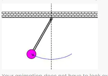
A straightforward pendulum comprises of mass which is appended by the line of length L from a turn point P. at the point when dislodged by beginning power the mass gets moved to and fro performing intermittent movement. By applying the Newton's

AIM : To write a program that solves the second order ODE which represents the equation of motion of a simple pendulum with damping.

THEORY :

In the above equation,

g = gravity in (m/s^2),

L = length of the pendulum in (m),

m = mass of the ball in (kg),

b=damping coefficient.

By substituting,

θ">θ

= θ1">θ1

d(θ1)dt">d(θ1)dt

= θ2">θ2

By solving above equation we get the solution set,

ddt[θ1θ2]">ddt[θ1θ2]

= [θ2-(bm)θ2-(gl)sinθ1]">[θ2−(bm)θ2−(gl)sinθ1]

CODE :

FUNCTION CODE :

function [dtheta_dt] = ode_func(t,theta,b,g,l,m)

theta1 = theta(1);
theta2 = theta(2);
dtheta1_dt = theta2;
dtheta2_dt = -(b/m)*theta2 - (g/l)*sin(theta1);
dtheta_dt = [dtheta1_dt; dtheta2_dt];

end

MAIN CODE :

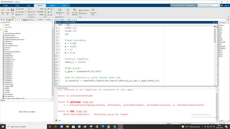
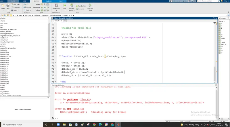
CODE EXPLANATION:

1. Clear all, close all, clc are used to clear the work space, to clear the graphs that’s exists, and clear the command window.
2. The inputs are for the simple pendulum are specified and the b = damping coefficient = 0.05 (n-m/s), g = acceleration due to gravity = 9.81 (m/s), l = length of the string = 1(m), m = mass of the bob = 1 (kg).
3. t_span is a command used in the ode45 solver which specifies the time span of the iterations that are going to solve the ordinary differential equation.
4. ode45 is a function in MATLAB that solves ordinary or partial differential equations using a numerical method. In this problem the highest order is 2. So, we have to take two constant values so that the equation is changed to simple differential equation.
   The function should take at least 2 inputs to solve the equation to the approximate result.
   The ode45 function has a syntax in which we need to specify which should be ‘t’ and ‘y’ and the output may be of (t, y, args) and a timespan for the function to work and the initial value of the equation.
   Syntax of a ode45 solver is,
   [t, results] = Ode45(@ (t, y) ode (t, y, args), t_span, y0).
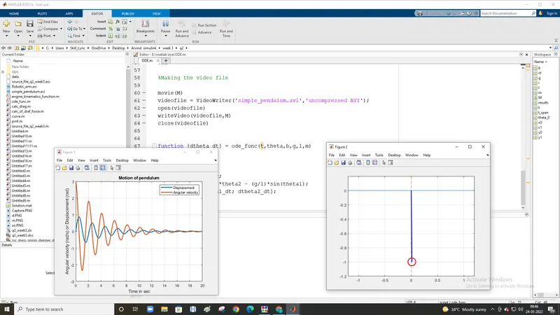
5. Figure (1) is going to tell how the damping is done for the pendulum. The angular velocity and displacement will come to rest at end of the function.
   Plotting the values for the angular velocity and the displacement by using plot command.
   The label command is used to label the X & Y axis.
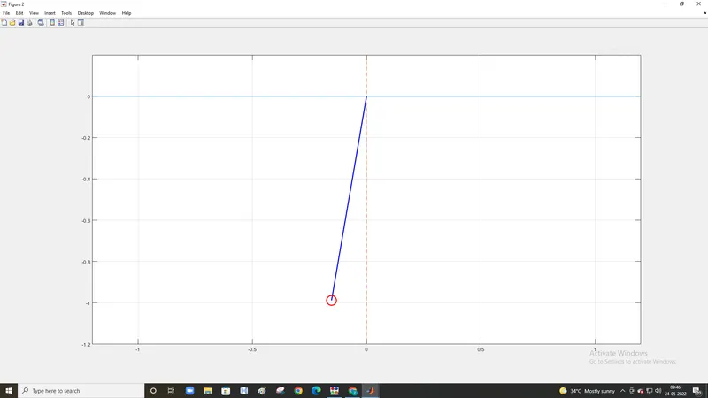
6. Legend command is used to label the angular velocity and the displacement.
   To animate the motion of simple pendulum, a for loop is used to create the specified set of points to keep the bob at different locations.
7. X0 and Y0 be the fixed point at one end of the string and x1 and y1 be the different position of the bob.
8. At each and every point of the bob the ‘ct’ command which is used to count all position and stores the data.
9. At the end of the for loop there will be set of positions for all points.
10. Movie(M) is used to create a film of the stored data of the motion of the pendulum.
11. videoWriter() command specifies the name of the file and type of data is stored in it.
12. Open() command is used to open the file where the video is going to store.
13. Writevideo() command is used to create the video animation by using M file.
14. Close() command is used to close the video file.

OUTPUT :

• Plot of angular velocity and displacement of simple pendulum with damping