Week 3 - Solving second order ODEs

Course: Python for Mechanical Engineers

Challenge: Solving Second-Order ODEs

Submitted By: Amanpreet Singh Whan

1 Aim:

The aim of the week 3 challenge is to write a program in python to solve second order Ordinary Differential Equation (ode).

2 Theory and Governing Equations:

The simple pendulum is another mechanical system that moves in an oscillatory motion. It consists of a point mass ‘m’ suspended using a light inextensible string of length L from fixed support as shown in Fig 1. The motion occurs in a vertical plane and is driven by a gravitational force. The forces which are acting on the mass are shown in the figure. The tangential component of the gravitational force, mg sin θ, always acts towards the mean position θ = 0 opposite to the displacement, restoring force acting tangent to the arc.

In Engineering, ODE is used to describe the transient behavior of a system. A simple example is a pendulum. The way the pendulum moves depends on Newton’s second law. This law derives a second-order Ordinary Differential Equation that describes the position of the ball of the pendulum w.r.t time.

Simple Pendulum

The free-body diagram of a simple pendulum in motion is represented by the following figure1.

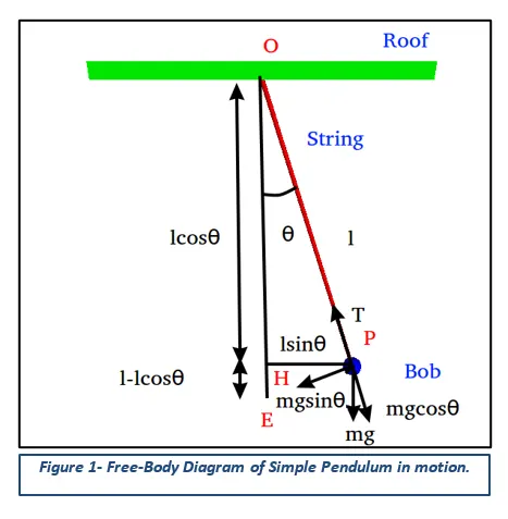
L = 1 m is the length of the pendulum.

m = 1 kg is the mass of the ball.

b = 0.05 is the damping coefficient.

g = 9.81 m/s^2 is the gravity.

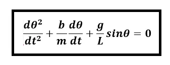
The ODE that represents the equation of motion of a simple pendulum with damping is as follows:

3 Objectives:

The objectives of the week 3 challenges are as follows:

• Write a program that can solve 2^nd order ODE and simulate the simple motion of the pendulum for 20 seconds.
• Create an animation file for the obtained results using the “Image Magick” software for the same.

4 Body of the Content:

Python is an interpreted, object-oriented, high-level programming language with dynamic semantics. Its high-level built-in data structures, combined with dynamic typing and dynamic binding, make it very attractive for Rapid Application Development and use as a scripting or glue language to connect existing components. Python's simple, easy-to-learn syntax emphasizes readability and therefore reduces the cost of program maintenance. Python supports modules and packages, which encourages program modularity and code reuse.

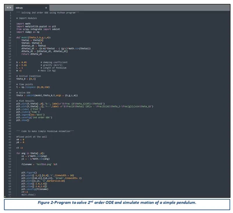
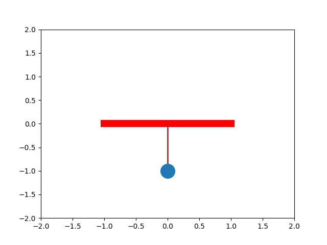
The python code was written to fulfill the requirements of the Week 3 challenge and is attached in the following figures. In addition, the animation created from the plots obtained from the written code is attached as well.

Simple Pendulum Animation

5 Conclusion:

In conclusion, the main aim of the week 3challenge is to write a python program to solve second-order Ordinary Differential Equation. In addition, create an animation file from the obtained plots using “ImageMagick” software.

6 Appendix:

''' Solving 2nd order ODE using Python program'''

# Import Modules

import math
import matplotlib.pyplot as plt
from scipy.integrate import odeint
import numpy as np

def model(theta,t,b,g,L,m):
	theta1 = theta[0]
	theta2= theta[1]
	dtheta1_dt = theta2
	dtheta2_dt = -(b/m)*theta2 - ( (g/L)*math.sin(theta1))
	dtheta_dt = [dtheta1_dt, dtheta2_dt]
	return dtheta_dt


b = 0.05           # damping coefficient
g = 9.81           # gravity (m/s^2)
L = 1              # Length of Pendulum
m =1             # Mass (in kg)

# Initial Condition
theta_0 = [0,3]

# Time points
t = np.linspace (0,20,150)

# Solve ODE
theta = odeint(model,theta_0,t,args = (b,g,L,m))

# Plot Results
plt.plot(t,theta[:,0],'b-', label=r'$\frac {d\theta_1}{dt}=\theta2$')
plt.plot(t,theta[:,1],'r--',label =r'$\frac{d\theta2} {dt}= - \frac{b}{m}\theta_2-\frac{g}{L}sin\theta_1$')
plt.ylabel ('Plot')
plt.xlabel('time')
plt.legend(loc='best')
plt.savefig('2nd order ODE')
plt.show()



''' Code to make Simple Pendulum Animation'''

#fixed point at the wall
x0 = 0
y0 = 0

ct =1 

for ang in theta[:,0]:
	x1 = L*math.sin(ang)
	y1 = - L*math.cos(ang)

	filename = 'test%5d.png' %ct
	

	plt.figure()
	plt.plot([-1,1],[0,0],'r',linewidth = 10)
	plt.plot([x0,x1],[y0,y1], 'brown',linewidth= 2)
	plt.plot(x1,y1, 'o',markersize=20)
	plt.xlim([-2.0,2.0])
	plt.ylim([-2.0,2.0])
	plt.savefig(filename)
	ct+=1
	#plt.show()