Week 3 - Solving second order ODEs

Aim :

To solve second order differential equation by using MATLAB

Objective :

To write the program code for solving second order equation, which represents the motion of a simple pendulam with damping.

Theory :

ODE means an ordinary differential equation and it is a differential equation containing one or more functions of one independant variable and derivatives of its functions.

Simple Pendulum is an idealized mathematical model of a pendulum. This is a bob on the end of a massless cord suspended from a pivot, without friction. When giving an intial force, it will be moving in to and fro motion. The way the pendululm moves depends on the Newtons second law. When this law is written down, we get a second order ODE that describes the position of the ball with respect to time. Similarly, there are hundreds of ODEs that describe key phenomena.

Formula

`(d^2theta)/(dt)^2 +(b/m). (d theta)/dt +(g/L) .sin(theta) =0`

where,

g is gravity in metre per second square,

L is length of pendulum in m,

m is mass of the ball in kg,

b is damping coefficient,

theta is angle of the pendulum with horizontal

Procedure :

• Firstly, the given input parameters are assigned as variables in the program code.
• Time span of the simple pendulum is set by using linspace command that is from 0 to 20s with 500 points between them.
• We use ode45 function and corresponding 'ode_funct' function call in main program.
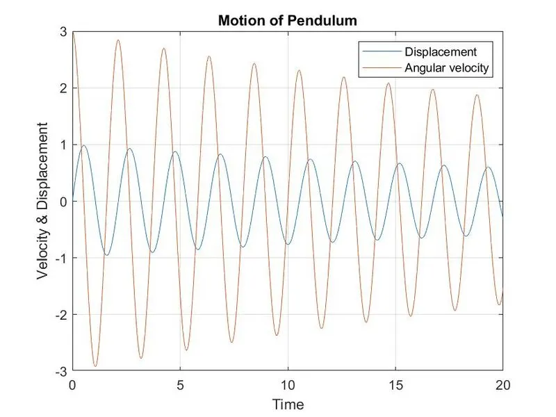
• Plot command is used to plot graph corresponding to time and velocity, legend command is used for identifying.
• Using the for loop command the mass at various points and various times are marked and motion of the pendulum is animated.
• Marker command is used for making bob of the pendulum. The axis is fixed using axis command.
• Then videoWriter command is used to create the video file.

Main Code :

clear all
close all
clc

% Input parameters

b = 0.05; % Damping co-efficient
g = 9.81; % Acceleration due to gravity(m/s^2)
m = 1; %  mass in kg
l = 1; % length in meters
 
% Initial condition
theta_0 = [0;3];
 
% Time points
tspan = linspace(0,20,500);
 
% Solving ode
[t,results ]= ode45(@(t,theta) ode_funct(t,theta,b,g,l,m),tspan,theta_0);
 
% Plotting of Angular velocity and displacement
figure(1)
plot(t,results(:,1))
hold on
plot(t,results(:,2))
grid on
title('Motion of Pendulum')
xlabel('Time')
ylabel('Velocity & Displacement')
legend('Displacement','Angular velocity')
angle = results(:,1);
saveas(1,'Velocity time diagram.jpg')
% Count command for iterations
ct = 1;
for i = 1:length(results(:,1))
    omega = angle(i);
    
    x0 = 0;
    y0 = 0;
    x1 = 1*sin(results(i,1)+pi);
    y1 = 1*cos(results(i,1)+pi);
    figure(2)
    M(ct) = getframe(gcf);
   
    % Plotting of the bob motion
    plot([x0 x1],[y0 y1],'linewidth',3,'color','g');
    hold on
    plot(x1,y1,'o','markers',10,'MarkerFaceColor','r');
    hold on
    plot([-3 3],[0 0],'linewidth',3,'color','b');
    hold off
    axis([-3 3 -2 2])
    title('Motion of pendulum')
    grid on
    pause(0.01)
    M(ct) = getframe(gcf);
    ct = ct+1;
end
 
%Movie and creating videofile in mp4
movie(M)
v_f = VideoWriter('Simple_pendulum_challenge.mp4','MPEG-4');
open(v_f)
writeVideo(v_f,M)
close(v_f)
    
    
    
    

Function Code :

% Ode function
function dtheta_dt = ode_funct(t,theta,b,g,l,m);
theta1 = theta(1);
theta2 = theta(2);
dtheta1_dt = theta(2);
dtheta2_dt = -(b/m)*theta2-(g/l)*sin(theta1);
dtheta_dt = [dtheta1_dt; dtheta2_dt];
end

Results :

1. Graph for the velocity vs time which shows Displacement and angular velocty:

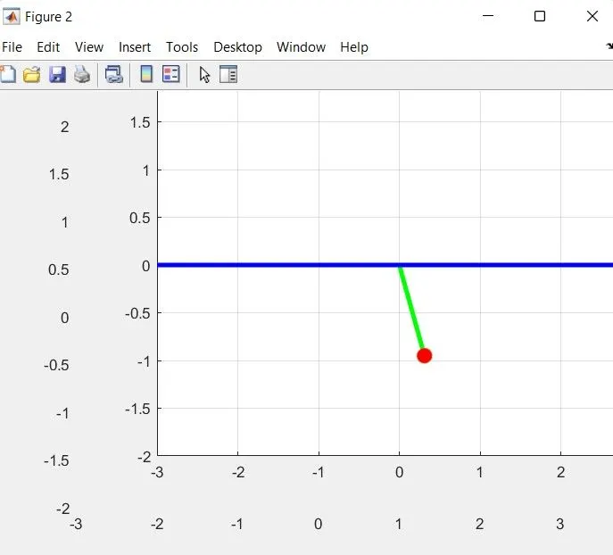
2. Position of the setup:

3. Youtube link of animation :

https://youtu.be/PZoM047k6Fs

Conclusion :

1. The graph of Displacement and Angular velocity is plotted in velocity vs Time diagram.

2. Animation of simple pendulum is created.

Error :

No major errors were found.