Project 2 - Rankine cycle Simulator

Aim :

To create a Rankine cycle simulator using Matlab and plot the corresponding T-S and H-S diagram for the given sets of inputs.

Objective :

To create a Rankine cycle simulator and calculate all the state points in it. And plot of T-S and H-S diagram for the inputs given in the question.

Rankine Cycle :

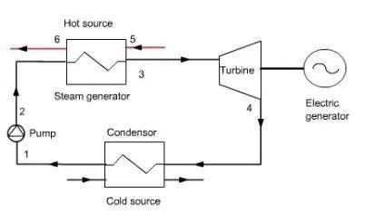
Rankine is an ideal thermodynamic cycle, here by moving a fluid between a heat source and heat sink a mechanical work is extracted, such as steam turbines or reciprocating steam engines. Heat is supplied through a boiler and their high-pressure gas forms and it will run the turbine. After running the turbine, the gas goes to the condensor part where it rejects all the heat and condenses. Then this fluid is again taken to the boiler through a pump. In rankine cycle there are four processes, they are:

• Process 1-2: The working fluid is pumped from low to high pressure. As the fluid is a liquid at this stage, the pump requires little input energy. Process 1-2 is isentropic comopression.
• Process 2-3: The high-pressure liquid enters a boiler, where it is heated at constant pressure by an external heat source to become a dry saturated vapour.Process 2-3 is constant pressure heat addition in boiler.
• Process 3–4: The dry saturated vapour expands through a turbine, generating power. This decreases the temperature and pressure of the vapour, and some condensation may occur.
• Process 4–1: The wet vapour then enters a condenser, where it is condensed at a constant pressure to become a saturated liquid. Process 4-1 is constant pressure heat rejection in condenser.

Main Code :

clear all
close all
clc
%displaying rankine cycle simulator and its processes
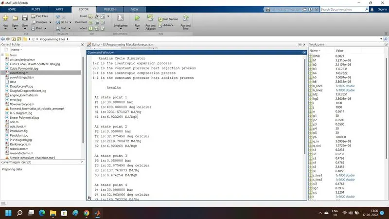
disp("   Rankine Cycle Simulator")
fprintf('1-2 is the isentropic expansion process')
fprintf('\n2-3 is the constant pressure heat rejection process')
fprintf('\n3-4 is the isentropic compression process')
fprintf('\n4-1 is the constant pressure heat addition process')
 
% State variables At state point 1
p1=30;
t1=400;
h1=XSteam('h_pT',30,400);
s1=XSteam('s_ph',30,h1);
fprintf('\n\n       Results')
fprintf('\n\n At state point 1')
fprintf('\n P1 is:%f bar',p1)
fprintf('\n T1 is:%f deg celcius',t1)
fprintf('\n H1 is:%f KJ/Kg',h1)
fprintf('\n S1 is:%f KJ/KgK',s1)

% State variables At state point 2
p2=0.05;
s2=s1;
t2=XSteam('T_ps',0.05,6.1858);
sf2=XSteam('sL_p',p2);
sg2=XSteam('sV_p',p2);
hf2=XSteam('hL_p',p2);
hg2=XSteam('hV_p',p2); 
x=((s2-sf2)/(sg2-sf2));
h2=hf2+(x*(hg2-hf2));
v2=XSteam('v_ph',p2,h2);
fprintf('\n\n At state point 2')
fprintf('\n P2 is:%f bar',p2)
fprintf('\n T2 is:%f deg celcius',t2)
fprintf('\n H2 is:%f KJ/Kg',h2)
fprintf('\n S2 is:%f KJ/KgK',s2)

% State variables At state point 3
p3=p2;
t3=t2;
h3=XSteam('hL_T',32.875);
s3=XSteam('sL_p',p3);
v3=XSteam('v_ph',p3,h3);
fprintf('\n\n At state point 3')
fprintf('\n P3 is:%f bar',p3)
fprintf('\n T3 is:%f deg celcius',t3)
fprintf('\n H3 is:%f KJ/Kg',h3)
fprintf('\n S3 is:%f KJ/KgK',s3)

% State variables At state point 4
p4=p1;
s4=s3;
v4=v3;
h4=XSteam('h_ps',p4,s4);
t4=XSteam('T_hs',h4,s4);
fprintf('\n\n At state point 4')
fprintf('\n P4 is:%f bar',p4)
fprintf('\n T4 is:%f deg celcius',t4)
fprintf('\n H4 is:%f KJ/Kg',h4)
fprintf('\n S4 is:%f KJ/KgK',s4)

% State variables At state point 5
p5=p4;
t5=XSteam('Tsat_p',p5);
h5=XSteam('hL_T',t5);
s5=XSteam('sL_p',p5);
fprintf('\n\n At state point 5')
fprintf('\n p5 is:%f bar',p5)
fprintf('\n T5 is:%f deg celcius',t5)
fprintf('\n H5 is:%f KJ/Kg',h5)
fprintf('\n S5 is:%f KJ/KgK',s5)

% State variables At state point 6
t6=t5;
p6=XSteam('psat_T',t5);
h6=XSteam('hV_T',t6);
s6=XSteam('sV_T',t6);
fprintf('\n\n At state point 6')
fprintf('\n P6 is:%f bar',p6)
fprintf('\n T6 is:%f deg celcius',t6)
fprintf('\n H6 is:%f KJ/Kg',h6)
fprintf('\n S6 is:%f KJ/KgK',s6)

%loop to find variables on saturation lines
t=linspace(0,400,1000);
for i=1:length(t)
    s_line1(i)=XSteam('sL_T',t(i));
end

for j=1:length(t)
    s_line2(j)=XSteam('sV_T',t(j));
end
for i=1:length(t)
    h_line1(i)=XSteam('hL_T',t(i));
end 

for j=1:length(t)
    h_line2(j)=XSteam('hV_T',t(j));
end


%net work output calculation
w_turbine=h1-h2;
w_pump=h4-h3;
work=w_turbine-w_pump;
q_in=h1-h4;
q_out=h2-h3;

%thermal efficiency
n=work/q_in;

%back work ratio
BWR=w_pump/w_turbine;

%specific steam consumption
ssc=3600/work;

%plottin T-s graph
figure(1)
hold on
plot([s_line1 s_line2],[t t])
plot([s1 s2 s3 s4 s5 s6 s1],[t1 t2 t3 t4 t5 t6 t1])
text(s1,t1,'1')
text(s2,t2,'2')
text(s3,t3,'3')
text(s4,t4,'4')
text(s5,t5,'5')
text(s6,t6,'6')
title('Rankine Cycle T-S diagram')
xlabel('Entropy(KJ/KgK)')
ylabel('Temperature(K)')
legend ('Saturation Curve','location','North')
axis([0,8,0,450])
saveas(1,'T-S diagram.jpg')

%plotting h-s graph
figure(2)
hold on
plot([s_line1 s_line2],[h_line1 h_line2])
plot([s1 s2 s3 s4 s5 s6 s1],[h1 h2 h3 h4 h5 h6 h1])
text(s1,h1,'1')
text(s2,h2,'2')
text(s3,h3,'3')
text(s4,h4,'4')
text(s5,h5,'5')
text(s6,h6,'6')
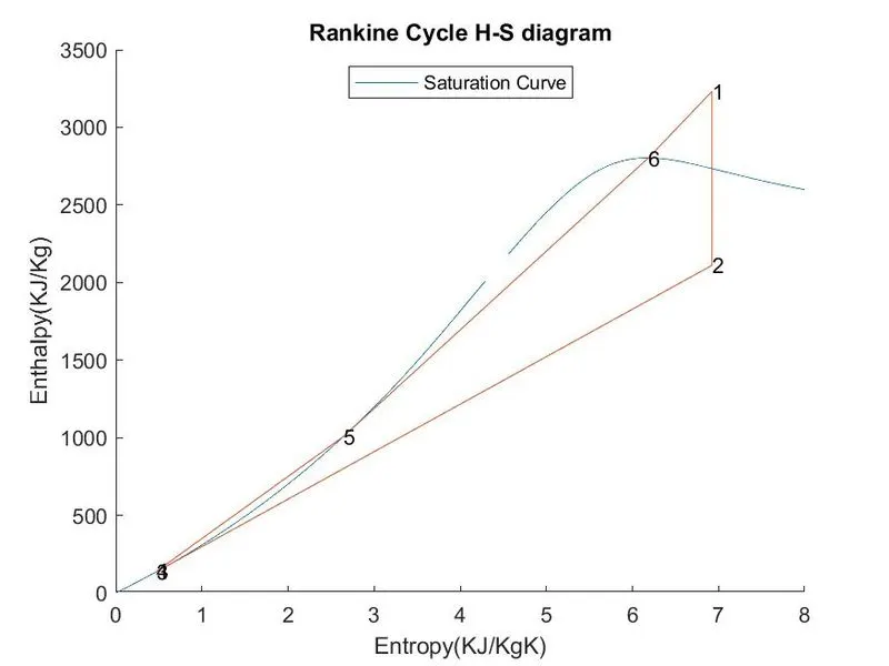
title('Rankine Cycle H-S diagram')
xlabel('Entropy(KJ/KgK)')
ylabel('Enthalpy(KJ/Kg)')
legend ('Saturation Curve','location','North')
axis([0,8,0,3500])
saveas(2,'H-S diagram.jpg')

Procedure :

• First of all use clear all,close all and clc for clearing workspace data, clearing plots and figures and to clear data in the command window.
• Using disp command we will display "Rankine cycle simulator" and then followed by all the proccess occuring in a rankine cycle which is dispalyed using fprintf command.
• Now we find the state variables at each point. The turbine inlet pressure, p1 is taken as 30 bar and inlet temperature is taken as 400K and turbine outlet temperature is taken as 0.05bar.
• We will put XSteam.m file in the same path and call the XSteam function to find respective state point values.
• XSteam data is used to extract steam and water properties of enthalpy, entropy at specific pressure and temperatures for sat liquid, sat vapour conditions etc.
• The XSteam data works as, h1 = XSteam('h_pT', p1,t1) ; which will be returning the enthalpy of water at given pressure and temperature in bar and degC.
• As we extract the data, we use thermodynamic relation to further find state points and extract their data from XSteam.
• sf and sg, hf and hg, where f and g stands for saturated liquid and saturated vapour respectively.
• The net work, work done by turbine, work done to run the pump, Heat in and heat out are calculated using standard thermodynamic relation.
• After finding each state point variables we will use fprintf command to display the results in the command window.
• We use for loop to find the values of enthalpy and entropy at saturated temperature and store them into variables.
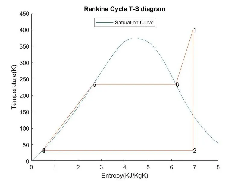
• At last, we will plot the graph of T-S and H-S diagram from all the values that we obtained from the above procedure.
• Saturation curve is plotted for saturated liquid and saturated gas.
• Saveas command is used for saving the plot figures.
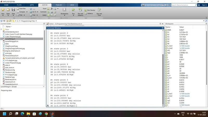
• Results are displayed in the command window.

Result :

Plots of T-S and H-S diagram

Results in Command window :