Week 3 - Solving second order ODEs

SIMULATING A SIMPLE PENDULUM

The following input conditions were used: 

• Acceleration due to gravity, g = 9.8 m/s^2
• Damping coefficient, b = 0.05 (we can vary this value and observe pendulum behaviour).
  
• Mass, m = 1 Kg 
• Length of pendulum, L = 1 m
• Initial conditions: 
  • Time period, t = 0 to 20 s
  • Angular displacement, Theta = 0 rad (at t = 0)
  • Angular Velocity, d(Theta)/dt = 3 rad/sec

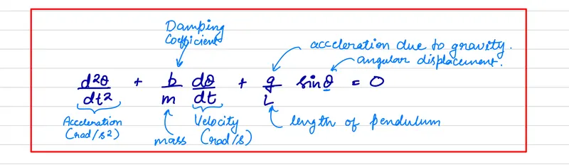
In order to solve this second order ODE, we will first convert it into a set (or, system) of first order ODE equations, as shown in the derivation below: 

  

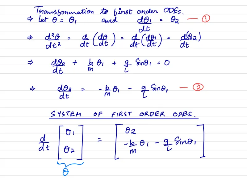
Note the column representation provided in the end. We will create column vectors in exactly the same format in order to be able to solve the ODEs using one of MATLAB's inbuilt solvers. Now that we have a set of first order ODEs, we can proceed to write a MATLAB program with the following logic/steps: 

1. Initialize the input variables and the intial conditions. 
2. Write a function 'ode_func' containing the first order equations. 
3. Utilize the inbuilt solver 'ode45' to provide the initial conditions/inputs. The solver will spit out two outputs, namely t & results. 
   • 't' is column vector containing all the time values b/w 0 to 20 seconds. Its length depends on the resolution provided by the user. 
   • 'results' is a matrix with two columns. The first column contains the displacement values, and the second column contains the angular velocities.  
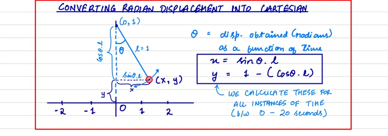
4. It must be noted that in order to plot the position of the pendulum in cartesian coordinates, we need to convert the radian displacment values to cartesian coordinates(refer the following sketch): 
   • 
   • Extract the displacement values (in radians) from the 'results' matrix into a column vector disp_radians.
   • Use the formulae shown in the sketch above to create row vectors 'x' & 'y' containing the cartesian cordinates for all the corresponding values of disp_radians & time (t). 
5. Use the data stored in x & y vectors to plot the pendulum position using a for loop. 
   • The for loop will repeat(iterate) for all the values of time b/w 0 - 20 s. 
   • For each iteration, we will plot the position (basically a single point) of the pendulum. We can also connect it to fixed point above it with a straight line in order to simulate its string.
   • We then capture this position (or, plot image) into a matrix M. 
6. Once the for loop ends, we can stitch all the images stored in M using the movie command, and store it with desired filename and video profile. 

The ode45 solver: 

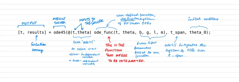
The ode45 solver is one of the many solvers available in MATLAB. The following is a brief description of its syntax: 

• [t, results] - The solver returns a solution matrix 'results', where each row correspond to the time returned in 't'. Since we have two first order ODEs, we have two columns in the 'results' matrix.
• @(t, theta) tells the solver that our ODEs are a function of time(independent variable) and theta(dependent variable). Note that 'theta' containes two columns since we have a system of two first order ODEs. 
• 'ode_func' is the user defined function that takes 't', 'theta', as well as 'b', 'l', 'm' and 'g' as inputs and returns the system of first oder ODEs in the format shown in the image above.
• 't_span' tells the solver the time span over which it needs to integrate the function. 
• 'theta_0' provides the intitial conditons (or the start points) for our ODE. Essentially, this means the we will plot the behaviour of the pendulum from this starting condition. There can be several different initial conditions that can be provided. 

ode45 essentially takes the time span and the initial condition vectors, passes them on to the user defined function (ode_func) which generates a system of first order ODEs based on these inputs. These first order ODEs are then integrated over t_span and returns a solution array 'results' corresponding to each values in the the time array 'y'. 

Code: 

%CHALLENGE #6 | WEEK 3 | SOLVING SECOND ORDER ODEs
%DHANANJAY PATEL | 11 APR 2022

tic;                    %times the program runtime(start)
clear all;
close all;
clc;

%Inputs 

%Acceleration due to gravity | m/s^2
g = 9.82;
%Damping coefficient
b = 0.05;
%Length | meters
l = 1;
%Mass | Kg
m = 1;


%Initial conditions
theta_0 = [0;3];                %Initial Dispalcement & Velocity
t_span = linspace(0,20,500);    %Time interval & time step

%Solve ODE

[t, results] = ode45(@(t,theta) ode_func(t, theta, b, g, l, m), t_span, theta_0);

%Extract the displacment valus from the results matrix.
disp_r = results(:, 1);

%Define fixed point of pendulum, x & y coordinates
x_p = 0;            
y_p = 3;


%Initialize x & y vectors to store coordinates of the pendulum location for
%each value of the time, t.
x = zeros(length(t_span), 0);
y = zeros(length(t_span),0);

%Radians to cartesian conversion 
x = sin(disp_r).*l;
y = y_p - (cos(disp_r).*l);

counter = 1;          

%For loop to plot & store several images of the pendulum.
for i = 1:length(t)
    
    hold on;
    %Plot the pendulum string
    plot([x_p x(i)], [y_p y(i)], 'LineWidth', 3);

    %Plot the pendulum position (single point)
    plot(x(i), y(i), '-O', 'MarkerSize',20, 'MarkerEdgeColor','red', 'MarkerFaceColor',[1 .6 .6]);
    
    %Define axis, label, title, and relevant text/information
    axis([-1 1 1.5 3]);
    xlabel('X Axis, m');
    ylabel('Y Axis, m');
    title('Second Order ODE - Simulating Pendulum Motion ');

    legendText1 = sprintf('Damping Coefficient (b) = %.3f', b);
    legendText2 = sprintf('Time step (delta t) = %.3f seconds' , t_span(2) - t_span(1));
    legendText3 = sprintf('Time interval = %.1f to %.1f seconds' , t_span(1), t_span(end));
    textbox = sprintf('%s\n%s\n%s', legendText1, legendText2,legendText3);
    text(0, 1.65, textbox);
    
    pause(0.02);

    %Store plot image from the current figure into M.
    M(counter) = getframe(gcf);
    counter = counter + 1;
   
    %stringth length is just to cross check if the (x,y) coordinates for the
    %pendulum have been computed correctly. It should compute the same value
    %for any pair of (x,y) coordinates. 
    string_length(i,1) = (((x(i)-x_p)^2 + (y(i)-y_p)^2)^2)^0.5;

    if i < length(t)
        clf;
    end
end

%Create a movie file by stichting all the images/frames stored in M
movie(M)
video_file = VideoWriter('Pendulum_ODE.avi', 'Uncompressed AVI');
open(video_file)
writeVideo(video_file, M)
close(video_file)

toc;            %Times the program runtime(end)

Function code: 

function [dtheta_dt] = ode_func(t, theta, b, g, l, m)

%theta has the initial conditions. Assign them to theta1 and theta2 to
%solve the ODEs
theta1 = theta(1);
theta2 = theta(2);

dtheta_dt = zeros(500, 2);

%Solving the first order ODEs
dtheta1_dt = theta2;
dtheta2_dt = -(b/m)*theta2 - (g/l)*sin(theta1);
dtheta_dt = [dtheta1_dt; dtheta2_dt];

end

Errors: 

1. The equation in line 33 is missing a pair of parantheses. Correction x = sin(displacement(i)); instead of x = sin(displacement(i); 

Note: the vector 'displacment' has since been renamed to 'disp_r'.

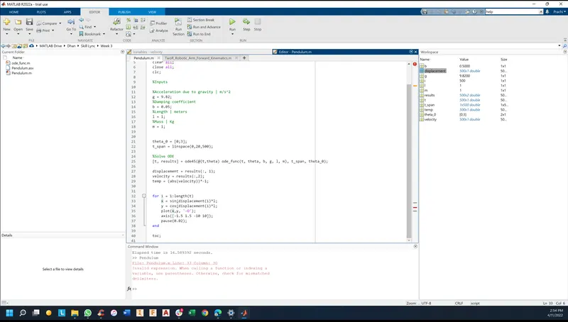
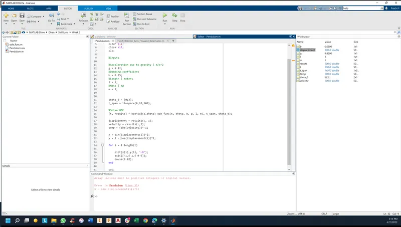
2. In the equation x = sin(displacement(i))*l, the displacement(i) vector did not logically make sense. Also the value for 'i' is not initialized until a few lines later when the for loop begins. 

The correct equation is x = sin(displacement)*i; (since the whole displacement vector needs to be utilized to get the all the cartesian coordinates for 'x' )

Note: the vector 'displacement' has since been renamed to 'disp_r'.  

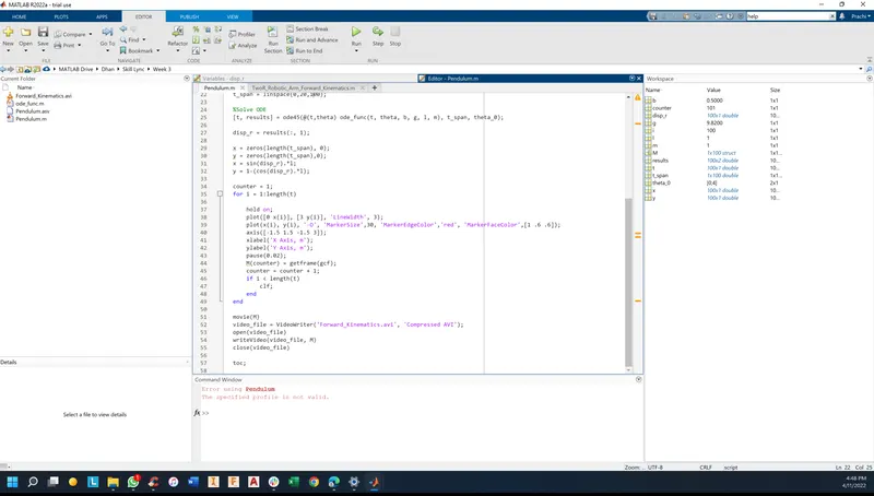
3. Video profile was incorrect. Correction -> 'Uncompressed AVI' instead of 'Compressed AVI'.

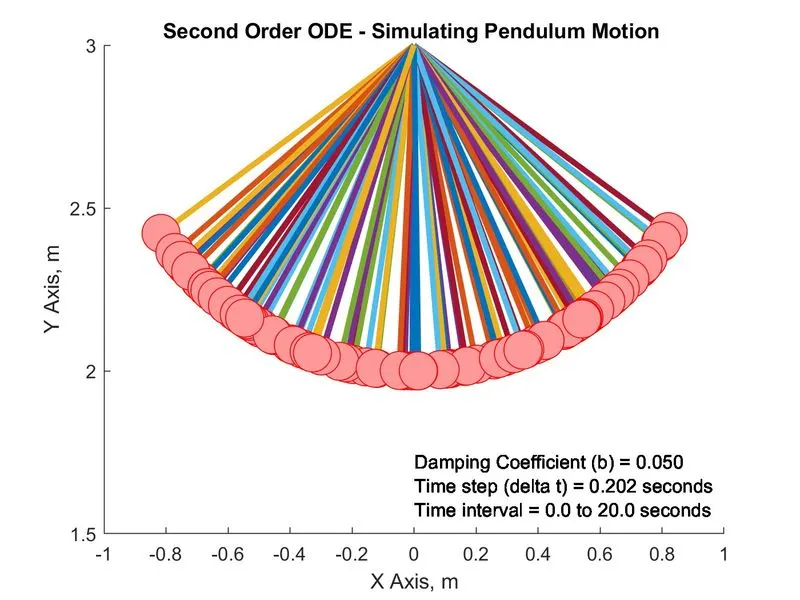
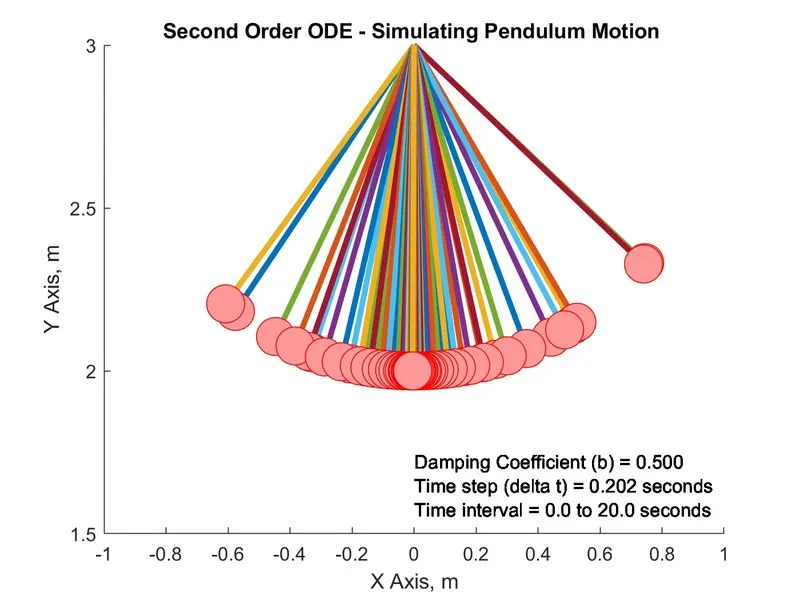
Output plot - Images: 

The following images show all the positions that the pendulum takes for different damping coefficient values. 

 

Output plot - animated videos: 

Following are the links to the videos showing the pendulum behaviour when the damping coefficient is changed.

Link1: Damping Coefficient = 0.05 

Pendulum ODE animation | Damping coefficient 0.05 - YouTube 

Link2:  Dampin Coefficient = 0.5

Pendulum ODE Animation | Damping Coefficient 0.5 - YouTube