AIR STANDARD CYCLE (OTTO CYCLE)

PLOTTING THE P-V DIAGRAM FOR AN IDEAL OTTO CYCLE

The Otto cycle is a thermodynamic cycle used to represent the processess in an Internal Combustion (IC) engine. Before we list down the major stages in an Otto Cycle, let us try to briefly understand the piston geometry:

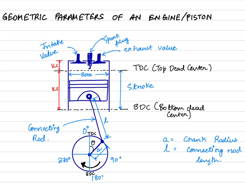
As seen from the sketch above, the piston is connected to the crankshaft via a connecting rod, and it moves up and down inside the piston cylinder/combustion chamber. At the top of the combustion chamber are intake & exhaust valves, as well as the spark plug, which provides ignition via a spark (a tiny arc-flash) at the appropriate instant. The highest and the lowest points that the piston can move to are known as Top Dead Center (TDC) and Bottom Dead Center (BDC) respectively. The kinematic equations for this piston will govern the PV diagram.

Now that we've described the basic piston arrangement, we shall discuss about the major processess in an Otto Cycle:

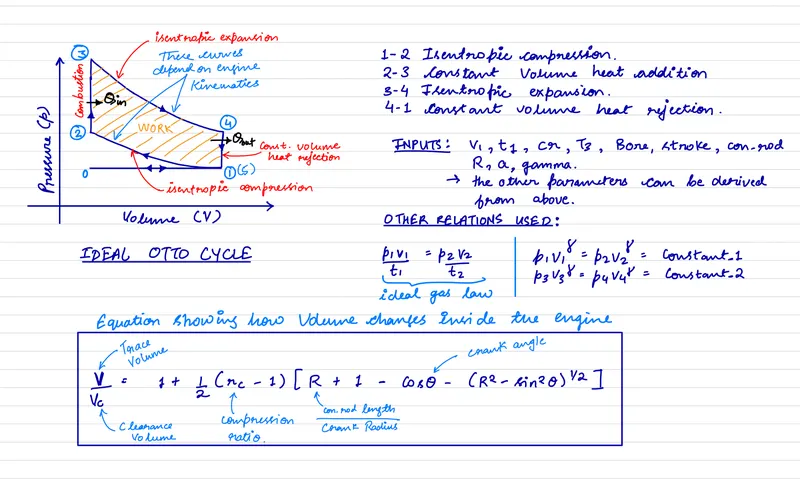
1. Air intake Stroke (0 -> 1): The air intake valve opens, air from the surroundings, along with fuel is sucked into the chamber as the piston moves from TDC to BDC.
2. Compression Stroke (1 -> 2): The air-fuel mixture is compressed by the piston (BDC to TDC). Work is done by the piston on the gas. The ideal process is adiabatic (no heat loss/transfer) and isentropic in nature. However, practically, there is some heat loss/transfer.
3. Combustion (2 -> 3): An accurately timed spark from the sparkplug ignites the air-fuel mixture, causing instantaneous combustion while the volume remains constant. In practical applications, this process is not constant-volume.
4. Expansion, or Power Stroke (3 -> 4): Rapid expansion of the ignited gas (air-fuel mixture) pushes the piston down. Work is done on the piston by the gas as it moves from TDC to BDC. This work (mechanical energy) is extracted to move the vehicle as well as power the ancillary systems in a vehicle.
5. Heat rejection (4 -> 1): The Exhaust valve opens at this point, and heat is rejected at a constant volume.
6. Exhaust stroke (5 -> 0): Piston moves from BDC to TDC, pushing the exhaust gases out thru' the exhaust valve.

MATLAB Program:

The PV diagram generated in this program more so represents the 'ideal' Otto cycle. In a practical scenario, the state transitions are not as sharp as shown here and have an overlap. Also, we shall not take the Air Intake Stroke (0 -> 1) and Exhaust Stroke (5 -> 0) into consideration for this program.

Steps:

• Calculate all the state variables at state points 1, 2, 3, & 4 respectively from the inputs provided.
  • The appropriate thermodynamic relations to obtain these variables (p1-p4, v1-v4, t1-t4) are used.
  • Plot the four state points: State points 1, 2, 3, & 4 respectively.
• Now, in order to connect state points 1->2 (isentropic compression) and 3->4 (isentropic expansion) with the right curve (it is not a straight line!), we shall utilize the geometric parameters of the piston.
  • The kinematic equation for the piston can be used to calculate the volume trace at a given crank angle, `theta`.
    • A separate MATLAB function, named piston_kinematics was written to calculate the volume trace.
  • Using this function, we can compute the arrays for v_compression (b/w crank angles 0 deg - 180 deg) & v_expansion (b/w crank angles 180 deg - 0 deg).
  • v_compression & v_expansion can be used to calculate the arrays for p_compression & p_expansion.
  • Plot the curves b/w state points 1->2 and 3->4 using (v_compression, p_compression) & (v_expansion, p_expansion).
• Since the processes b/w state points 2->3 and 4->1 are constant volume processes (in the ideal cycle), we simply connect them with a straigt line.
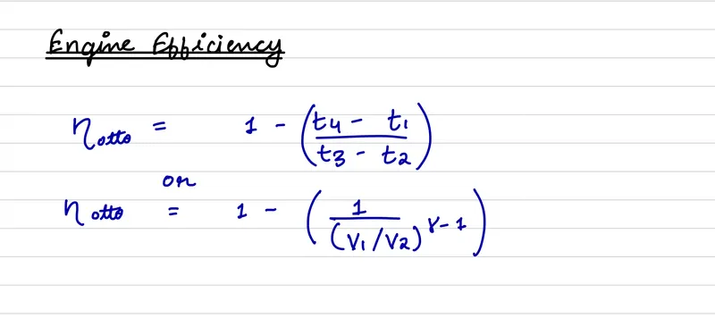
• In order to calculate the engine efficiency, we will simply utilize the state variables previously computed and plug them in the following equation.
• 

Code:

%CHALLENGE #5 | WEEK 2.1 | DHANANJAY PATEL | 6 APR 2022

%Program to create an Otto Cycle Plot and calculate engine efficiency. 

close all; 
clear all; 
clc;

%Inputs 
gamma = 1.4;
p1 = 101325; 
t1 = 500;       %Kelvin
t3 = 2300;      %Kelvin 

%Engine geometric parameters - dictate the variable volume process.

bore = 0.1;
stroke = 0.1;
con_rod = 0.15;         %connecting rod length, meters 
cr = 12;                %Compression Ratio
start_crank = 0;        %Starting crank angle
end_crank = 180;        %End crank angle

%Swept Volume and Clearance Volume
v_swept = (pi/4)*bore^2*stroke;
v_clearance = v_swept/(cr-1);

v1 = v_clearance + v_swept;
v2 = v_clearance;

%State variables at STATE POINT 2
%p1*v1^gamma = p2*v2^gamma - defines the isentropic compression process
%v1/v2 = cr 
p2 = p1*cr^gamma;

%Ideal gas law to compute t2
%(p1v1)/t1 = (p2v2)/t2
t2 = (p2/p1)*(1/cr)*t1; 

const_c1 = p1*v1^gamma;

%Function call to compute v_compression array
v_compression = piston_kinematics(bore, stroke, con_rod, cr, 180, 0);

p_compression = const_c1./(v_compression.^gamma);

%State variables at STATE POINT 3 - end point of constant volume combustion
%process. Therefore, v2 = v3. 

v3 = v2; 

%Use ideal gas law to compute p3. 
%p2v2/t2 = p3v3/t3  |   p3 = (p2*v2*t3)/(t2*v3);
p3 = (p2*t3)/t2;

const_c2 = p3*v3^gamma;

%Function call to compute v_compression array
v_expansion = piston_kinematics(bore, stroke, con_rod, cr, 0, 180);

p_expansion = const_c2./(v_expansion.^gamma);

%State variables at STATE POINT 4
v4 = v1; 

%(p3*v3)^gamma = (p4*v4)^gamma => p4 = p3(v3/v4)^gamma
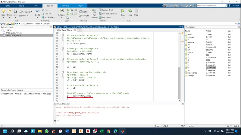
p4 = p3*(v3/v4)^gamma; 

%Calculating t4 using the ideal gas law. t4 will be used to compute the
%engine efficiency.
%p1*v1/t1 = p4*v4/t4
t4 = (p4*v4*t1)/(p1*v1);

%Plot 
figure(1)
hold on;
plot(v1,p1, '*', 'color','black');                          %State Point 1
plot(v_compression, p_compression, 'color', 'r');       %Isentropic Compression Curve
plot(v2,p2, '*', 'color','black');                          %State Point 2
plot([v2 v3], [p2 p3], 'color', 'b');                   %Const. vol. heat addition curve
plot(v3,p3, '*', 'color','black');                          %State Point 3
plot(v_expansion, p_expansion, 'color', 'g');           %Isentropic Expansion Curve
plot(v4,p4, '*', 'color','black');                          %State Point 4
plot([v4 v1], [p4 p1], 'color', 'b');                   %Const. vol. heat rejection        
xlabel('Volume, V');
ylabel('Pressure, P');
legend('', '1->2 Isentropic Compression', '', '2->3 Constant vol. heat addition.', '', '3->4 Isentropic Expansion', '', '4->1 Const. vol. heat rejection.', 'Location','northeast');
title('P-V Diagram for an Ideal Otto Cycle', 'LineWidth',4);

%Engine Efficiency

%Expression for thermal efficiency => 1 -[(t4-t1)/(t3-t2)]
%which can also be written as => 1 - [1/cr^(gamma-1)]
eta_otto = 1 - (1/cr^(gamma-1));
eta_otto2 = 1 -[(t4-t1)/(t3-t2)];
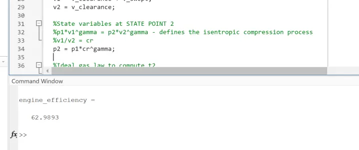
engine_efficiency = eta_otto*100

Function code:

function [v] = piston_kinematics(bore, stroke, con_rod, cr, start_crank, end_crank)

a = stroke/2;                       %Crank Radius
R = con_rod/a;                      

v_s = (pi/4)*bore^2*stroke;         %Swept volume 
v_c = v_s/(cr-1);                   %Clearance volume


theta = linspace(start_crank, end_crank, 180); 

%We split the kinematic equation of the piston to calculate the volume
%trace into three terms for simplicity during coding & ease of
%understanding
term1 = 0.5*(cr-1);
term2 = R + 1 - cosd(theta); 
term3 = (R^2 - sind(theta).^2).^0.5;

%Piston kinematic equation
%v -> volume trace
v = v_c.*(1 + term1*(term2 - term3));

end

Errors:

1. Typo Error: Undefined variable 'T1' -> corrected to 't1'

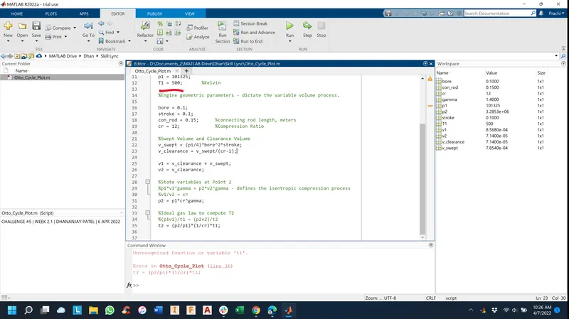
2. Typo error: Undefined variable 'p3' occurs both in LHS & RHS of the equation. Correction -> 'p3' was changed to 'p2' in the RHS of the equation.

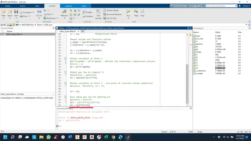
3. Syntax Error: multiplication operator '*' was missing in the equation. Correction -> add the multiplication operator '*' after 'p3'.

Output:

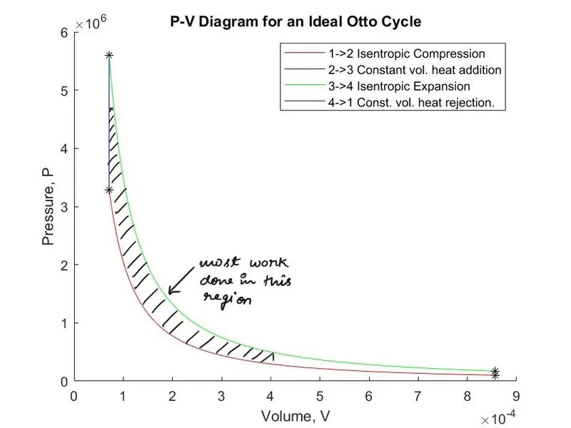
The following P-V diagram, and engine efficiency are displayed when we run the program.

Explanation of output plot:

1. The isentropic compression and isentropic expansion processes are not linear in nature, but rather depend on the engine/piston geometry. These processes are also adiabatic in nature for the ideal cycle - meaning there is no heat loss/tranfer, which is not the case in reality.
2. The constant volume heat additon (combustion) process is instantaneous. Agaain, this is not the case in reality, and there is indeed some change in the volume during combustion. Same applies for the constant volume heat rejection process.
3. We can also see that as the cyclinder approches the TDC during the compression stroke (1->2), it has to do a lot more work for even a small reduction in volume (simultaneosly causing a much steeper increase in the pressure).
4. Similarly, for the power stroke (3->4) most of the energy is transferred to the piston/crankshaft very rapidly (i.e high piston acceleration) at the early stages of the process, with very small amount of work being done as the piston approaches BDC.
5. This also shows the the engine output is not uniform during one complete cycle, and is provided in a short burst. To achieve a more balanced output, multiple pistons working at an 'offset' crank angles w.r.t. to each other are used. A flywheel is also used.

Note: Please refer this link showing the Real/Actual Otto Cycle.

Web sources used for research & information:

1. Main parameters of an engine piston and cylinder – x-engineer.org
2. Ideal Otto Cycle (nasa.gov)
3. 3.5 The Internal combustion engine (Otto Cycle) (mit.edu)