Week 3 - Solving second order ODEs

DETERMINING THE TRANSIENT BEHAVIOUR OF THE SIMPLE PENDULUM SYSTEM USING SECOND ORDER ORDINARY DIFFERENTIAL EQUATION (ODE)

ODE FUNCTION PROGRAM

The below ODE represents the equation of motion of a simple pendulum with damping

dθ² / dt² + (b/m) (dθ / dt) + g/l sinθ = 0

where,

g = acceleration due to gravity in m/s2,

L = length of the pendulum in m,

m = mass of the ball in kg,

b = damping coefficient.

Considering the angle theta = theta1 (θ = θ1) and differentiation of the angle theta1 = theta2 (dθ1 / dt = θ2) ,

which leads to dθ² / dt² = dθ2 / dt

So the equation can be simplified as mentioned in the below program

dtheta2_dt = -(b/m)*theta2 - (g/l)*sin(theta1)

function [dtheta_dt] = ode_func(t,theta,b,g,l,m)

theta1 = theta(1)
theta2 = theta(2)
dtheta1_dt = theta2
dtheta2_dt = -(b/m)*theta2 - (g/l)*sin(theta1);
dtheta_dt = [dtheta1_dt; dtheta2_dt];
end

ANGULAR DISPLACEMENT AND ANGULAR VELOCITY GRAPHS WTIH RESPECT TO TIME

clear all
close all
clc

x0 = 0;
y0 = 0;
b=0.05;
g=9.81;
l=1;
m=1;

% Initial condition
theta_0 = [0;3];

% time points
t_span = linspace(0,20,500);

% solve ODE
[t, results] = ode45(@(t,theta) ode_func(t,theta,b,g,l,m),t_span, theta_0);

figure(1)
plot(t,results(:,1))
hold on
plot(t,results(:,2))
ylabel('Plot')
xlabel('time')


y = results(:,1);
ct = 1;
for i = 1:length(t_span)

x0 = 0;
y0 = 0;
x1 = -l*sin(y(i));
y1 = -l*cos(y(i));

figure(2)

plot([x0 x1],[y0 y1],'linewidth',3,'color','r')
line([-1 1],[0 0],'linewidth',3,'color','g')
axis([-2 2 -2 2]);
grid on
hold on
plot(x0,y0,'o','markersize',3,'markerfacecolor','r');
plot(x1,y1,'o','markersize',20,'markerfacecolor','r');
pause(0.03)
M(ct) = getframe(gcf);
ct = ct+1;
clf
end

movie(M)

videofile = VideoWriter('Oscillating_Pendulum.avi','Uncompressed AVI');
open(videofile)
writeVideo(videofile,M)
close(videofile)

Consider the intial condition of the simple pendulum be

x0 = 0
y0 = 0
b = 0.05
g = 9.81
l = 1
m = 1

where,

x0 and y0 are the co-ordinates for the fixed end of the simple pendulum

g = acceleration due to gravity in m/s2,

l = length of the pendulum in m,

m = mass of the ball in kg,

b = damping coefficient.

theta_0 = [0;3]

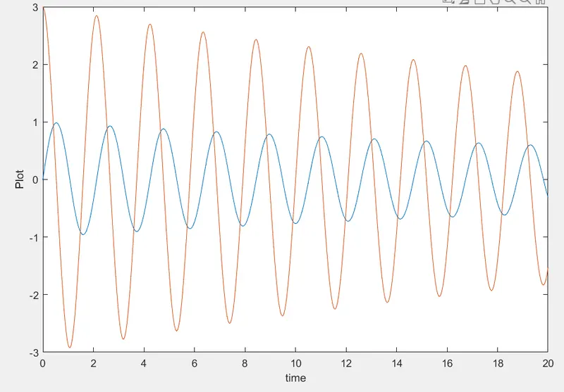
The above line represents the intial conditions of angular displacement = 0 and angular velocity = 3

t_span = linspace(0,20,500)

The above line represents the time span of oscillation of the simple pendulum from 0 sec to 20 secs.

[t, results] = ode45(@(t,theta) ode_func(t,theta,b,g,l,m),t_span, theta_0)

The above line executes the ODE by carrying the ode45 function

figure(1)
plot(t,results(:,1))
hold on
plot(t,results(:,2))
ylabel('Plot')
xlabel('time')

By the executing the above command where the Angular displacement and Angular velocity values are extracted and are used to plot the graphs with respect to Time

y = results(:,1);

The above line indicates that the Angular displacement values from the time span 0 to 20 secs are indicated by the variable 'y'

ct = 1;
for i = 1:length(t_span)

x0 = 0;
y0 = 0;
x1 = -l*sin(y(i));
y1 = -l*cos(y(i));

The initial x0 and y0 represents the fixed end of the simple pendulum, while x1 and y1 represents the oscillating end of the simple pendulum

figure(2)

plot([x0 x1],[y0 y1],'linewidth',3,'color','r')
line([-1 1],[0 0],'linewidth',3,'color','g')
axis([-2 2 -2 2]);
grid on
hold on
plot(x0,y0,'o','markersize',3,'markerfacecolor','r');
plot(x1,y1,'o','markersize',20,'markerfacecolor','r');
pause(0.03)
M(ct) = getframe(gcf);
ct = ct+1;
clf
end

The data obtained is used to plot multiple graphs for the respective time span using the above mentioned for loop

movie(M)

videofile = VideoWriter('Oscillating_Pendulum.avi','Uncompressed AVI');
open(videofile)
writeVideo(videofile,M)
close(videofile)

The multiple plots obtained are incorporated into an animated video using the above mentioned command under the name 'Oscillating_Pendulum'

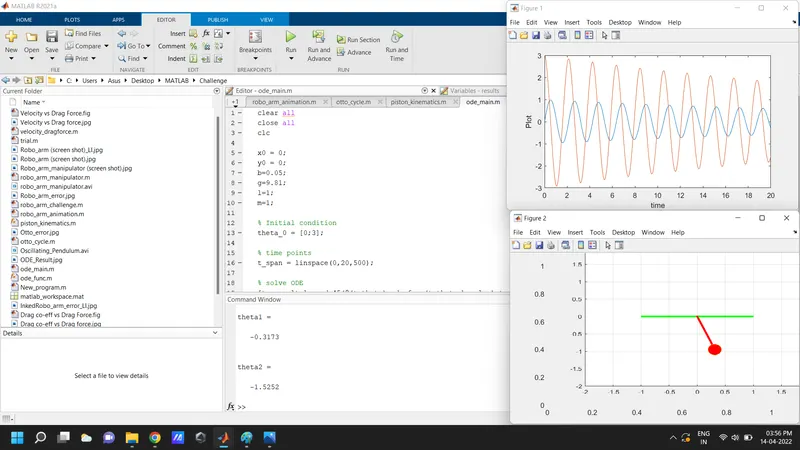
The animation of the Simple Pendulum for the above mentioned program is mentioned below

https://drive.google.com/file/d/1FlGOBPpe3Bf47V_UsL72iUCWR9TV85Fj/view?usp=sharing

ERRORS ENCOUNTERED

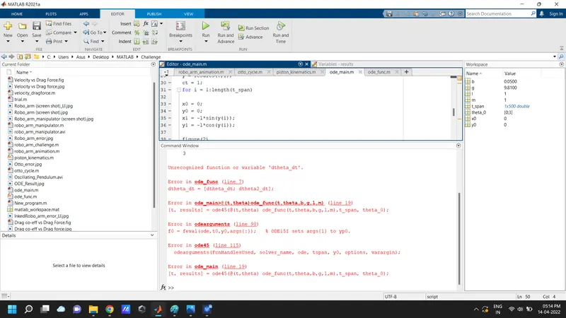
The error is due to the error in the line number 7 of the ode_func.

dtheta_dt = [dtheta_dt; dtheta2_dt];

CORRECTIVE ACTION

By correcting the error from line number 7 as mentioned below the required results can be obtained.

dtheta_dt = [dtheta1_dt; dtheta2_dt];