Week 3 - Solving second order ODEs

In this project objective is to write a program that solves the following ODE. This ODE represents the equation of motion of a simple pendulum with damping

Theory

The way the pendulum moves depends on the Newtons second law. When this law is written down, we get a second order Ordinary Differential Equation that describes the position of the "ball" w.r.t time.

Equation

We need to convert above complex eqn into simple one to generate the requried datad

d²θ1/dt + b/m*dθ1/dt + g/l*sin(θ1) = 0

dθ1/dt = θ2 .........eq.1

substitute eq.1 in above eq then

dθ2/dt + b/m*θ2 + g/l*sin(θ1) = 0

dθ2/dt = -b/m*θ2 - g/l*sin(θ1) ........eq.2

from using above two eq's write a code to solve the objective

import numpy as np 
from scipy.integrate import odeint 
import matplotlib.pyplot as plt
import math

# function that returns dz/dt
def model(theta,t,b,g,l,m):
	theta1 = theta[0]
	theta2 = theta[1]
	dtheta1_dt = theta2
	dtheta2_dt = (-b/m)*theta2 - (g/l)*math.sin(theta1)
	dtheta_dt = [dtheta1_dt, dtheta2_dt]
	return dtheta_dt

b = 0.05
g = 9.81
l = 1
m = 1

#initial condition
theta_0 = [math.pi/3, math.pi/2]

#time condition
t = np.linspace(0,20,150)

#line points
theta = odeint(model,theta_0,t,args = (b,g,l,m))

#plot result
plt.plot(t, theta[:,0])
plt.plot(t, theta[:,1])
plt.xlabel('time')
plt.ylabel('theta')
plt.title('ODE')
plt.savefig("ODE"+".png")
plt.show()

# animation
ct = 1

x0 = 0
y0 = 0

for i in theta[:,0]:
	x1 = (1*math.sin(i))
	y1 = (-1*math.cos(i))

	filename = 'test%5d.png' %ct
	ct = ct + 1

	plt.figure()
	plt.plot([-1,1], [0,0],"black",linewidth=8)
	plt.plot([x0,x1],[y0,y1], "red")
	plt.plot(x1,y1,'o',markersize=15)
	plt.xlim([-1.5,1.5])
	plt.ylim([-1.5,1.0])
	plt.savefig(filename)

Result

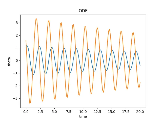
From the below graph it is shown that the anguler velocity and the angular displacement is decresing over time due to the dampers

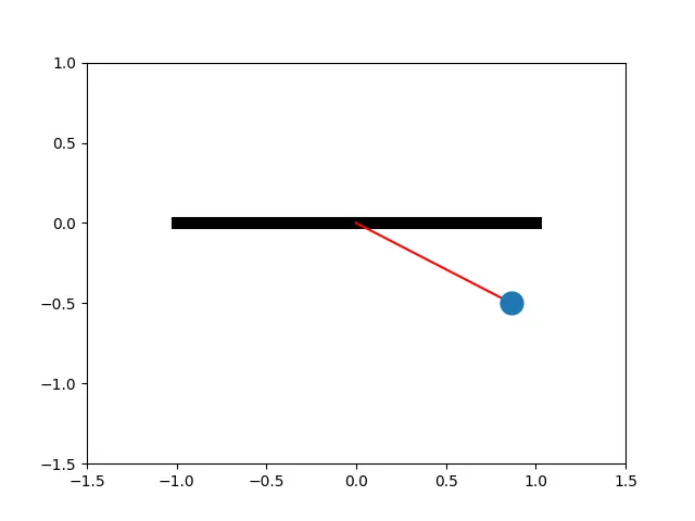
The animation of how pendulum works for different angles is shown below

YOUTUBE LINK: https://studio.youtube.com/video/O0PFot7FKLs/edit