Week 3 - Solving second order ODEs

Aim:

To create an animation of simple pendulum by using 2nd order differential equation by using ode solver function in MATLAB.

Theory:

A simple pendulum consists of a heavy metallic (brass) sphere with a hook (bob) suspended from a rigid stand, with clamp by a weightless inextensible and perfectly flexible thread through a slit cork, capable of oscillating in a single plane, without any friction, with a small amplitude (less than 150). There is no ideal simple pendulum. In practice, we make a simple pendulum by tying a metallic spherical bob to a fine cotton stitching thread.

The spherical bob may be regarded by as a point mass at its centre G. The distance between the point of suspension S and the centre G of the spherical bob is to be regarded as the effective length of the pendulum. The effective length of a simple pendulum, L = l + h + r. Where l is the length of the thread, h is length of hook, r is radius of bob.

The simple pendulum produces Simple Harmonic Motion (SHM) as the acceleration of the pendulum bob is directly proportional to its displacement from the mean position and is always directed towards it. The time period (T) of a simple pendulum for oscillations of small amplitude.

Inputs:

L = 1 m

m = 1 kg

b = 0.05

g = 9.81 m/s^2

time span = 0 - 20 secs

angular displacement = 0

angular velocity = 3 rad/s^2 (when t=0)

Program:

clear all
close all
clc

b=0.05;       % damping coefficient
g=9.81;       % gravity (m/s^2)
l=1;          % length of the pendulum (m)
m=1;          % mass of the bob (kg)

theta_0 = [0;2];             % initial condition
t_span = linspace(0,20,500); % time points for the pendulum oscillation

% solving ODE 

[t,results] = ode45(@(t,theta) ode_func(t, theta, b, g, l ,m), t_span, theta_0);

% plotting

figure(1)
plot(t, results(:,1)) 
hold on
plot(t, results(:,2))
xlabel("plot")
ylabel("time")

% For loop & animation plotting

ct = 1;
for i = 1:length(results(:,1))
    x_start = 0;
    y_start = 0;
    x_end = l*sin(results(i,1));
    y_end = -l*cos(results(i,1));
    figure(2)
    plot([-1,1],[0,0],'linewidth',3,'Color','red') % base of pendulum
    hold on
    plot([x_start x_end],[y_start y_end],"linewidth",4,"color",'black') % string of pendulum
    plot(x_end, y_end,'marker','o','MarkerSize',25,'MarkerFaceColor','y') %  bob of pendulum
    axis([-2 2 -2 2])
    pause(0.03)
    hold off
    M(ct)=getframe(gcf);
    ct=ct+1;
end

% movie creation

movie(M);
videofile = VideoWriter('simple_pendulum.avi','Uncompressed AVI');
open(videofile);
writeVideo(videofile,M);
close(videofile);

Funtion code:

function [dtheta_dt] = ode_func(t, theta, b, g, l, m)
theta1 = theta(1);
theta2 = theta(2);
dtheta1_dt = theta2;
dtheta2_dt = -(b/m)*theta2 - (g/l)*sin(theta1);
dtheta_dt = [ dtheta1_dt; dtheta2_dt];
end

Output:

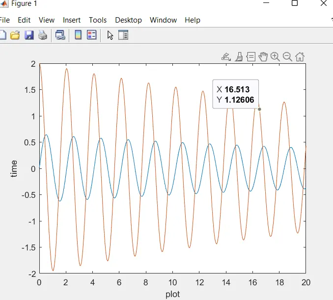
animation of the pendulum in the below link;

https://youtu.be/LI022bORVB8

Result:

Thus the animation of the simple pendulum was created by using MATLAB and uploaded in youtube successfully.