Week 3 - Solving second order ODEs

Aim: Solving second order ODEs

Theory -

The ordinary differential equation (or ODE) is a relation that contains functions of only one independent variable, and one or more of its derivatives with respect to that variable.

A simple example is Newton's second law of motion, which leads to the differential equation,

for the motion of a particle of mass m. In general, the force f depends upon the position of the particle x, and thus the unknown variable x appears on both sides of the differential equation, as is indicated in the notation f(x).

Ordinary differential equations are to be distinguished from partial differential equations where there are several independent variables involving partial derivatives.

OBJECTIVE OF THE PROJECT:

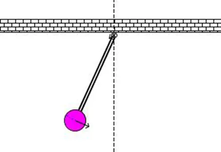
• The objective is to write a program that solves the following ODE. This ODE represents the equation of motion of a simple pendulum with damping
• Governing Equations.
• 

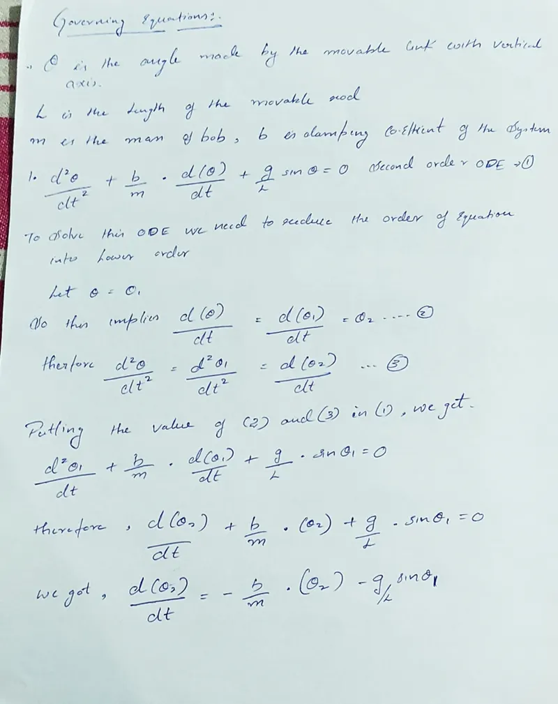
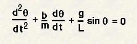
In the above equation,

g = gravity in m/s2,

L = length of the pendulum in m,

m = mass of the ball in kg,

b=damping coefficient.

Write a program in MATLAB\Octave that will simulate the pendulum motion, just like the one shown in the start of this challenge.

use,

L=1 metre,

m=1 kg,

b=0.05.

g=9.81 m/s2.

Simulate the motion between 0-20 sec, for angular displacement=0, angular velocity=3 rad/sec at time t=0.

MATLAB Code file

1. Code function of ODE45 for main program –

function [ dtheta_dt] = ode_func(t,theta,b,g,l,m)

theta1 = theta(1)

theta2 = theta(2)

dtheta1_dt = theta2;

dtheta2_dt = -(b/m)*theta2-(g/l)*sin(theta1);

dtheta_dt = [dtheta1_dt; dtheta2_dt];

end

2. Main program –

clear all

close all

clc

b=0.025; %damping coefficient

g=9.81; %length of pendulum in meter

l=1; %mass of bob in kg

m=0.1; %gravity in m/s^2

%initial condition

theta_0 = [0;5];

%time points

t_span = linspace(0,10,500);

%solve ODE

[t, results] = ode45(@(t,theta) ode_func(t, theta, b,g,l,m),t_span, theta_0);

plot(t,results(:,1))

hold on

plot(t,results(:,2))

ylabel('plot')

xlabel('time')

Code Explanation –

1. Firstly, the given details are assigned as variables in the code. Then time span of the simple pendulum is set by using linspace command then, theta value is given as a column matrix. After this, we use ODE45 function and corresponding ‘ODE_function’ Function call in the main program.

2. Then used the plot command to plot the graph corresponding to time and velocity, legend command is used to identify each value in the graph.

3. For getting the accurate simulation of the simple pendulum corresponding to the second-order ODE with damping we need to use the looping statements, here the loop is used to create this.

4. The pendulum has fixed coordinates mentioned as x0,y0, and x1,y1 is the other coordinates.

5. Marker command is used for making the bob of the pendulum. The axis is fixed using the axis command. The counter command is used to make the value changes in each for a loop. Then video writer command is used to create the video file.

Results-

Outputs

• Graph for the velocity V/s time which shows displacement and angular velocity

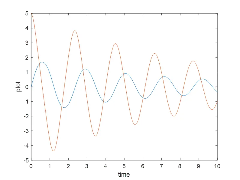
The displacement (blue color) and angular velocity (red color) is decreasing with the increased time, this is due to the introduction of damper I,e damping coeffect which absorbs the vibrations to make the body in equilibrium position

Conclusion

• The graph of displacement and angular velocity is plotted in the velocity Vs Time diagram.
• Animation of a simple pendulum is created.