Week 3 - Solving second order ODEs
ODE are used to solve complex problems where dependent and independent variables are used. but doing it manually requires knowledge of integration as well as the calculation is lengthy and that too limited asnwers are possible.
but,same if do it programically we get more range of data or solution set for ODE and it is time consuming.
following is the code for solving ODE in matlab,
INPUTS:
g = gravity in m/s2, g=9.81 m/s2
L = length of the pendulum in m, L=1 metre,
m = mass of the ball in kg, m=1 kg,
b=damping coefficient. b=0.05.
% SOLVING SECOND ORDER DIFFERENTIAL EQUATION BY PROGRAMMING IN MATLAB.
% INPUTS OF PENDULUM
l = 1;
m = 1;
b = 0.05;
g = 9.81;
% PENDULUM AT "T= O"(INITIAL POSITION)
disp_vcty = [0,3]; here (0) means the theta or displacement at inital position and(3) ,means initial velocity.
% TIME SPAN OF PENDULUM
t_span = linspace(0,20,600);
time span means how long we want to observe the displacement and velocity of bob w.r.t time.
[time,results] = ode45(@(t,theta) ode_function(t, theta,l,b,g,m),t_span,disp_vcty);
here, ode45 is inbuilt function in matlab for solving ODE. thus using it appropriately we will two data sets as time and results. time is simpl the t_span having 600 values and this function has integrated these 600 values w.r.t position and velocity.
because we have added a function named as "ode_function". we have saved this function in directory by converting the second order equation in two single order differential equations.
ODE_FUNCTION
function dtheta_dt = ode_function(t, theta, l,b,g,m)
theta1 = theta(1);
theta2 = theta(2);
dtheta1_dt = theta2;
dtheta2_dt = -(b/m)* theta2 - (g/l) * sin(theta1);
dtheta_dt = [dtheta1_dt ; dtheta2_dt];
end
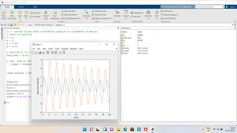
finally , after getting all the positions of bob w.r.t time ,we will plot graph for displacement, velocity, and time.
figure(1);
plot(time,results(:,1))
hold on
plot(time,results(:,2))
xlabel('time')
ylabel('disp and velocity')
ANIMATION CODE FOR PENDULUM :
l = 1;
ct =1;
for i = 1:length(t_span)
x0 = 0 ;
y0 = 0 ;
x1 = l.*sin(results(i,1));
y1 = -l.*cos(results(i,1));
figure(2)
plot([x0 x1],[y0 y1],'color','b','linewidth',3)
hold on
plot(x1,y1,'o','MarkerFaceColor','red','MarkerSize',15,'markerEdgecolor','red')
hold off
axis([-1 1 -1 1])
pause(0.03)
M(ct) = getframe(gcf);
ct = ct +1;
end
movie(M)
videofile = VideoWriter('simplependulum.avi','Uncompressed AVI');
open(videofile)
writeVideo(videofile,M)
close(videofile)
by fixing one end of pendulum as (0,0), we will set x1 and y1. but fixing (x1,y1) cannot be fixed ,since its not static and bob is under motion every second. so we can find position of bob at any one point out of all the points in motion of bob. now we know this completely depends upon the velocity and displacement of bob w.r.t time, thus creating a for loop will help us to find an matrix array for(x1,y1).
after getting all values we will be putting them alltogether to form a movie clip[, because initally they all are in frames, putting all frames together is animation . using above commands we can animate the bob position, velocity w.r.t time.
ABOVE CODE WAS RAN IN MATLAB AND RESULT IS OBTAINED AS VIDEOFILE , WHICH WAS UPLOADED ON YOUTUBE.
YOUTUBE LINK FOR VIDEO: https://youtu.be/GtgV-ik7P6g