Week 3 - Solving second order ODEs

Aim : Write a program in Python that will simulate the pendulum motion .

In mathematics, Ordinary Differential Equation (ODE) is a differential equation containing one or more functions of one independent variable and the derivatives of those functions

In Engineering, ODE is used to describe the Transient Behaviour of system Here, motion of Simple Pendulum is also governing by Second Order ODE as below

`(d^2theta) /dt^2 + b/m (d theta)/dt +g/L sin theta = 0`

where ,

           `theta` = Angular displacement 

             t = time (s)

             b = Damping coefficient

             m = Mass of Ball (kg)

            L = Length of string (m)

            g = Gravity (m/s^2)

Program : 

import numpy as np
from scipy.integrate import odeint
import matplotlib.pyplot as plt
import math

# function that return dz/dt
def model(theta,t,b,g,l,m):

    theta1 = theta[0]
    theta2 = theta[1]
    dtheta1_dt = theta2
    dtheta2_dt = -(b/m)*theta2 - (g/l)*math.sin(theta1)
    dtheta_dt = [dtheta1_dt, dtheta2_dt]
    return dtheta_dt

# inputs
b = 0.02
g = 9.81
l = 1
m = 0.1

# initial condition
theta_0 = [math.pi/2,0]

# time points
t = np.linspace(0,10,150)

# solve ode
theta = odeint(model,theta_0,t,args = (b,g,l,m))

# plot results
plt.plot(t,theta[:,0],'b-',label=r'$\frac{d\theta_1}{dt}=\theta2$')
plt.plot(t,theta[:,1],'r--',label=r'$\frac{d\theta2}{dt}=-\frac{b}{m}\theta_2-\frac{g}{l}sin\theta_1$')
plt.ylabel('plot')
plt.xlabel('time')
plt.legend(loc='best')
plt.show()

ct = 1
for Theta in theta[:,0]:
    x0 = 0
    y0 = 0

    x1 = l*math.sin(Theta)
    y1 = -l*math.cos(Theta)

    filename = str(ct)+ 'png'
    ct = ct+1

    plt.figure()
    plt.plot([-0.5,0.5],[0,0],'g',linewidth=5)
    plt.plot([x0,x1],[y0,y1],'r')
    plt.plot(x1,y1,'o',markersize=30)
    plt.xlim(-1.5,1.5)
    plt.ylim(-1.5,1.5)
    plt.title('animation of simple pendulum')
    plt.savefig(filename)

Output :

1) Graph -

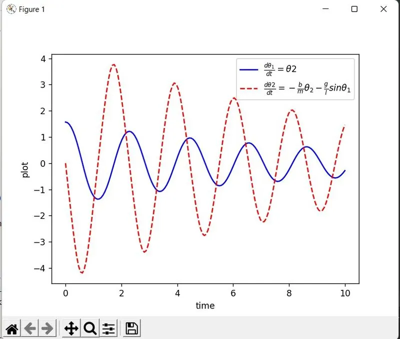
2) 150 pendulum images : 

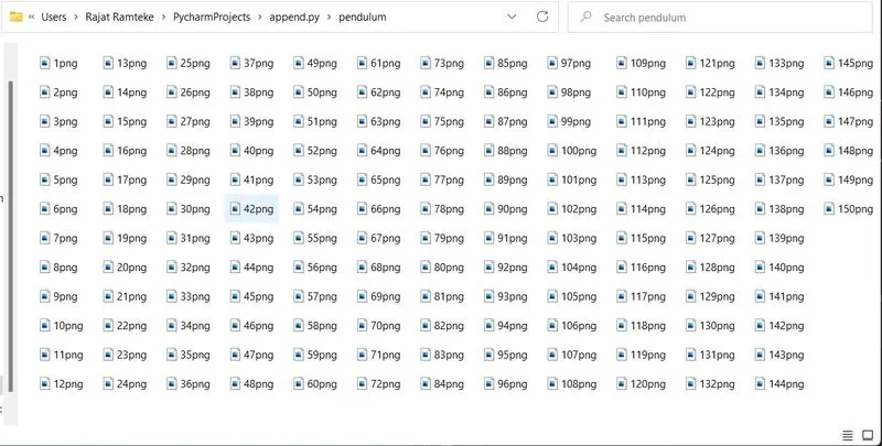
After getting 150 pendulum motion images , we have to to convert png images to gif animation . this animation attached in attachment .