Project 2 - Rankine cycle Simulator
Aim :- Create a Rankine Cycle Simulator using OCTAVE/MATLAB.
Calculate : - 1] Net work output
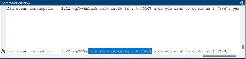
2] Back work ratio
PROGRAM :
close all
clear all
clc

% rankine cycle simulator
while(1)

    fprintf('RANKINE CYCLE SIMULATOR n');
    disp('process 1-2: Reversible Adiabatic expansion in turbine');
    disp('process 2-3: constant pressure hear rejection in condenser');
    disp('process 3-4: reversible adiabatic compression in pump');
    disp('process 4-1: constant pressure heat addition in boiler');

    % P1 = inlet pressure of turbine (bar)
    % P2 = outlet pressure of turbine (bar)
    % T1 = inlet temperature of turbine(degree c)

    fprintf('n')
    P1 = input('Enter pressure at turbine inlet(in bar): ');
    T1 = input('Enter temperature at turbine inlet(in degree celcius): ');
    P2 = input('Enter pressure at turbine outlet(in bar): ');

    % calculating state variable at point 1
    H1 = XSteam('h_pt',P1,T1);
    S1 = XSteam('s_pt',P1,T1);
    Hf1 = XSteam('hL_p',P1);
    Hg1 = XSteam('hV_p',P1);
    Ts1 = XSteam('Tsat_p',P1);
    Sf1 = XSteam('sL_p',P1);
    Sg1 = XSteam('sV_p',P1);

    % calculating state variable at point 2
    S2 = S1;
    Sf2 = XSteam('sL_p',P2);
    Sg2 = XSteam('sV_p',P2);
    x = (S2- Sf2)/(Sg2-Sf2);
    Hf2 = XSteam('hL_p',P2);
    Hg2 = XSteam('hV_p',P2);
    H2 = Hf2 +x*(Hg2-Hf2);
    T2 = XSteam('T_ph',P2,H2);
    Ts2= XSteam('Tsat_p',P2);

    % calculating state variable at point 3

    H3 = Hf2;
    S3 = Sf2;
    T3 = T2;
    P3 = P2;

   % calculating state variable at point 4
   P4 = P1;
   S4 = S3;
   H4 = XSteam('h_ps',P4,S4);
   T4 = XSteam('T_ps',P4,S4);

   t = linspace(0,374,500);

   % plot T-S diagram
   figure(1)
   hold on

   % plotting the saturation curve
   for i = 1:length(t)
       plot(XSteam('sL_T',t(i)),t(i),'.','Color','r');
       plot(XSteam('sV_T',t(i)),t(i),'.','Color','r');
   end

   % plotting the rankine cycle
   b1 = plot([S1 S2],[T1 T2],'LineWidth',1,'Color','b');
   if x>1
       T3=Ts2;
       b2 = plot([S2 Sg2 S3],[T2 Ts2 T3],'LineWidth',1,'color','m');
       T2 = Ts2;
   else

       b2 = plot([S2 S3],[T2 T3],'LineWidth',1,'Color','m');
   end

   b3 = plot([S3,S4],[T3,T4],'Color','k');

   b4 = plot([S4 Sf1 Sg1 S1],[T4 Ts1 Ts1 T1],'LineWidth',1,'Color','g');

   axis([0 15 -5 (T1+200)])
   xlabel('specific entropy [KJ/Kg-K]')
   ylabel('temperature[K]')
   legend([b1,b2,b3,b4],{'isentropic expansion in turbine','isobaric heat rejection in condensor','reversible adiabatic compression in pump','isobaric heat addition in boiler'},'Location','northeast');
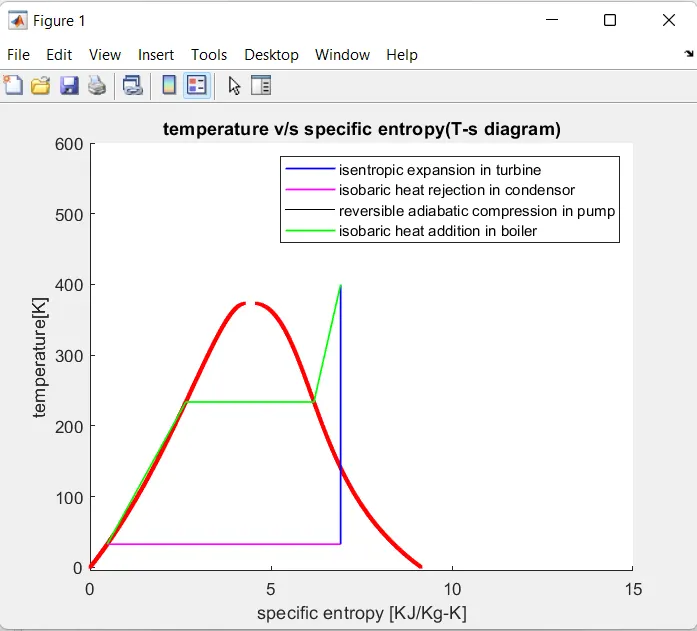
   title('temperature v/s specific entropy(T-s diagram)')
   hold off

   % plotting the H-S diagram
   figure(2)
   hold on
   % plotting the saturation curve
   for i = 1:length(t)
       plot(XSteam('sL_T',t(i)),XSteam('hL_T',t(i)),'.','Color','r')
       plot(XSteam('sV_T',t(i)),XSteam('hV_T',t(i)),'.','Color','r')
   end

   % plotting the rankine cycle
   a1 = plot([S1,S2],[H1,H2],'Color','b');
   a2 = plot([S2,S3],[H2,H3],'Color','g');
   a3 = plot([S3,S4],[H3,H4],'Color','k');
   a4 = plot([S4,S1],[H4,H1],'Color','m');
   xlabel('specific entropy [KJ/Kg-K]')
   ylabel('specific enthalpy [KJ/Kg]')
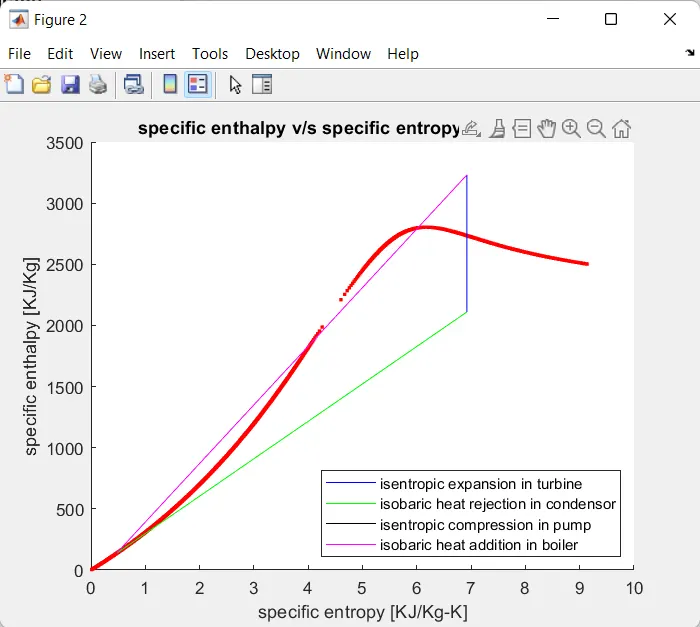
   title('specific enthalpy v/s specific entropy (H-S diagram)')
   legend([a1,a2,a3,a4],{'isentropic expansion in turbine','isobaric heat rejection in condensor','isentropic compression in pump','isobaric heat addition in boiler'},'location','southeast');
   hold off

   % calculations

   % turbine work
   Wt = H1-H2;

   % pump work
   Wp = H4-H3;

   % heat addition
   Qin  = H1-H4;

   % heat rejection
   Qout = H2-H3;

   % net work
   Wnet = Wt-Wp;

   %efficiency
   Ntherm = (Wnet/Qin)*100;

   % specific steam consumption
   SSC = 3600/Wnet;

   % back work ratio
   BWR = Wp/Wt;

   % printing results
   fprintf('n results')
   fprintf('parameters at state point 1:n')
   fprintf('P1 is : %.2f barn',P1)
   fprintf('T1 is : %.2f deg celcius',T1)
   fprintf('H1 is : %.2f KJ/kgn',H1)
   fprintf('S1 is : %.2f KJ/kg-kn',S1)

   fprintf('parameters at state point 2:n')
   fprintf('P2 is : %.2f barn',P2)
   fprintf('T2 is : %.2f deg celcius',T2)
   fprintf('H2 is : %.2f KJ/kgn',H2)
   fprintf('S2 is : %.2f KJ/kg-kn',S2)


   fprintf('parameters at state point 3:n')
   fprintf('P3 is : %.2f barn',P3)
   fprintf('T3 is : %.2f deg celcius',T3)
   fprintf('H3 is : %.2f KJ/kgn',H3)
   fprintf('S3 is : %.2f KJ/kg-kn',S3)

   fprintf('parameters at state point 4:n')
   fprintf('P4 is : %.2f barn',P4)
   fprintf('T4 is : %.2f deg celcius',T4)
   fprintf('H4 is : %.2f KJ/kgn',H4)
   fprintf('S4 is : %.2f KJ/kg-kn',S4)


   fprintf('n turbine work is : %.2f KJ/Kgn',Wt)
   fprintf('pump work is : %.2f KJ/Kgn',Wp)
   fprintf('work net (shaft work) is : %.2f KJ/Kgn',Wnet)
   fprintf('thermal efficiency is : %.2f percentn',Ntherm)
   fprintf('specific steam consumption : %.2f kg/KWhn',SSC)
   fprintf('back work ratio is : %.5f n',BWR)

   % assking if the user wants to continue
   fprintf(' ')
   x = input('do you want to continue ? [Y/N]: ','s');
   x = upper(x);
   if x == 'N'
       disp('n end for the rankine cycle simulator')
       break;
   else
       continue;
   end

end
Output : 1] T-S diagram
2] H-S Diagram
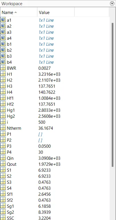
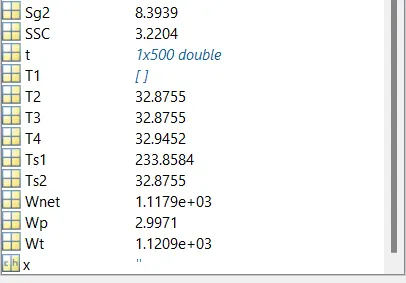
workspace :-
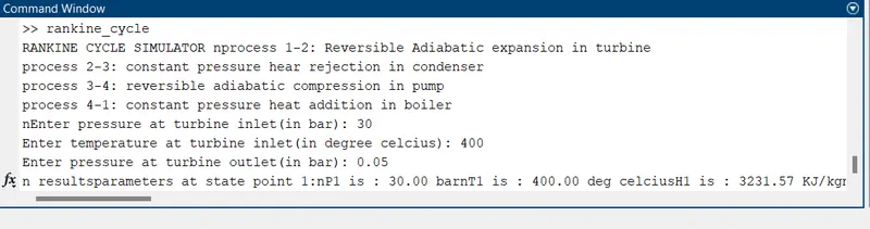
command window :
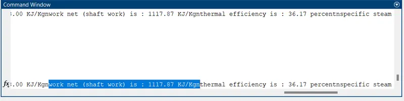
OUTPUT :-
1) Back work ratio
2) Net work output