Week 3 - Solving second order ODEs

In Engineering, ODE is used to describe the transient behavior of a system. A simple example is a pendulum

The way the pendulum moves depends on the Newtons second law. When this law is written down, we get a second order Ordinary Differential Equation that describes the position of the "ball" w.r.t time.

Similarly, there are hundreds of ODEs that describe key phenomena and if you have the ability to solve these equations then you will be able to simulate any of theses systems.

objective:-

write a program that solves the following ODE. This ODE represents the equation of motion of a simple pendulum with damping.

EXPLAINATION:-

ODE represents the transient behaviour of simple pendulum. Here, the ODE is second order differential equation but to solve in matlab we are breaking into two first order differential equation.

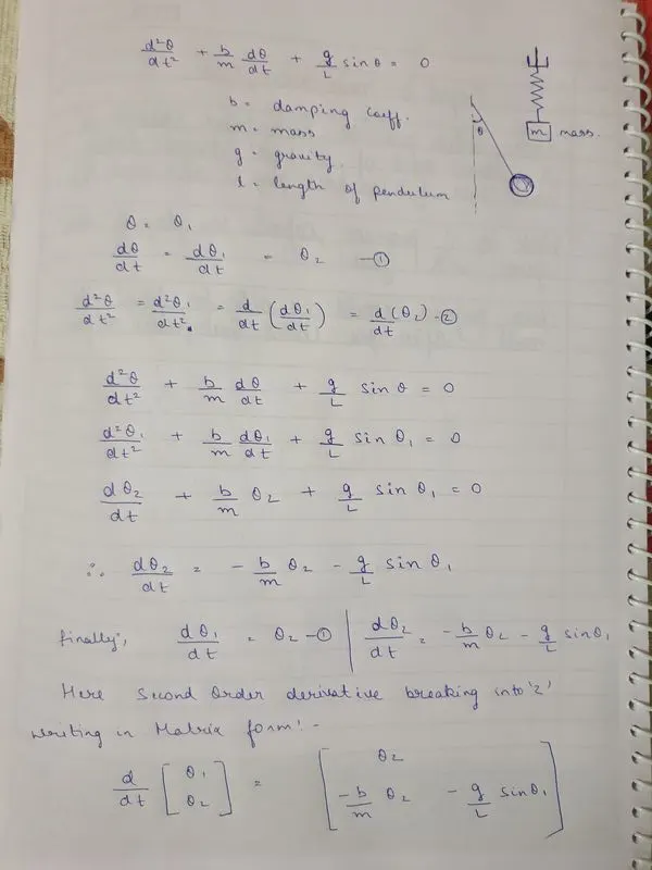
writing the above equation in matrix form:-

`d/dt[theta_1; theta_2] = [theta_2;-b/mtheta_2 -g/lsintheta_1]`

Program in Matlab that will simulate the pendulum motion:-

%Write a program in Matlab\Octave that will simulate the pendulum motion, just like the one shown in the start of this challenge.
%use,
%L=1 metre   - lengthof pendulum
%m=1 kg      - mass of bob
%b=0.05      - damping coeff.
%g=9.81 m/s2 - gravity
%Simulate the motion between 0-20 sec, for angular displacement=0,angular velocity=3 rad/sec at time t=0.

clc
clear all
close all

b=0.05
g=9.81
l=1
m=1


%initial condition
%theta is storing two values one for angular displacement and other is
%angular velocity:-

theta_0 = [0;3];

%time points
%time spann between 0 to 20 and inbetween there will be 200 values:-
t_span=linspace(0,20,200);

%solve ODE:-
%ode is the standard solver in matlab to solve the differential
%equation which gives the output of t and results.
%results are angular dispalcement and angular velocity which are stored in size 500x2 rows x column vector.
%first row is angular dispalcemnt and second is angular velocity.

[t, results] = ode45(@(t,theta) ode_func(t, theta, b,g,l,m),t_span,theta_0);

%PLOTTING:-
plot(t,results(:,1));
hold on;
plot(t,results(:,2));
xlabel('TIME');
ylabel('ANGULAR DISPLACEMENT AND ANGULAR VELOCITY');
legend('ANGULAR DISDPLACEMENT','ANGULAR VELOCITY');

Explaination:-

Input values of the following:-

b=0.05
g=9.81
l=1
m=1

theta_0 = [0;3];

Here, theta is storing two values angular displacement and angular velocity.

and then calculate ,

time span- with the help of linspace command

t_span=linspace(0,20,200) calculate 200 values.

with the help of ode solver in matlab and ode function input calculate ,

[t, results] = ode45(@(t,theta) ode_func(t, theta, b,g,l,m),t_span,theta_0);

then plot time and angular displacement and angular velocity.

FUNCTION COMMAND FOR SIMPLE PENDULUM:-

function[dtheta_dt]= ode_func(t,theta,b,g,l,m)

theta1 = theta(1);
theta2 = theta(2);
dtheta1_dt = theta2;
dtheta2_dt = -(b/m)*theta2 - (g/l)*sin(theta1);
dtheta_dt = [dtheta1_dt;dtheta2_dt];
end

Explaination:-

The above code is the function for solving simple pendulum eqn.

ANIMATION PROGRAM FOR SIMPLE PENDULUM:-

%ANIMATION OF PENDULUM:-
ct=1;
for i=1:length(t_span)
    x_fixed = 0;
    y_fixed = 0;
    x_freeend = 1*sin(results(i,1));
    y_freeend =-1*cos(results(i,1));

    plot([x_fixed x_freeend],[y_fixed y_freeend],[5 -5],[0 0])
    hold on
    plot(x_freeend,y_freeend,'marker','o','markerSize',30,'MarkerFaceColor','r')
    axis([-1.5 1.5 -1.5 1.5])
    hold off
    M(ct)=getframe(gcf)
    ct=ct+1;
end
movie(M)
videofile = VideoWriter('ode_pendulum.avi','Uncompressed AVI');
open(videofile)
writeVideo(videofile,M)
close(videofile)

Explainantion:-

Here i am animating the simple pendulum with the help of movie command:-

Initially keep ct(frame)=1 above for loop;

then by using for loop , calculate x_freeend and y_freeend with the help of

for i= 1:length(t_span)

put x_freeend=1*sin(results(i,1));

and y_freeend=-1*cos(results(i,1));

then plot x_fixed x_freeend y_fixed and y_freeend.

and then create movie by usual movie commands.

OUTPUT GRAPHS:-

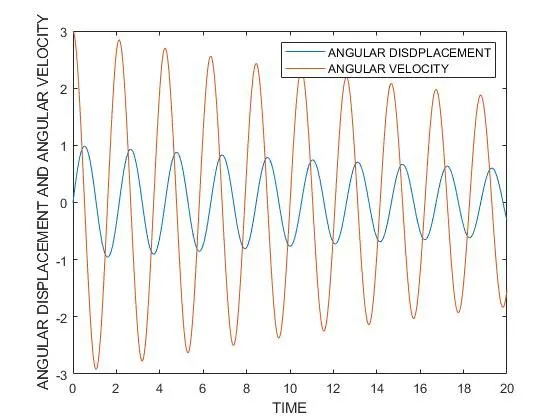
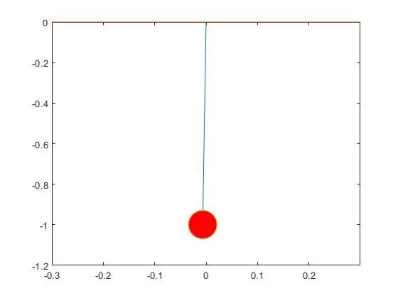
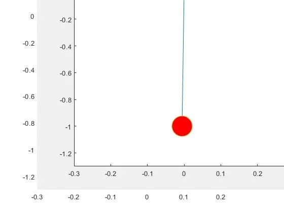
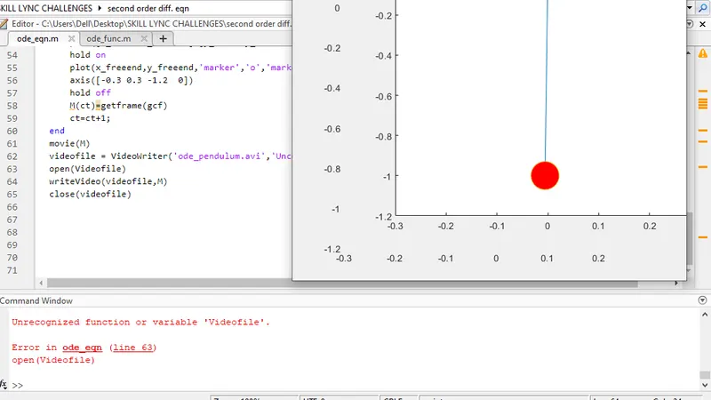
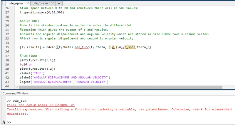
ERRORS WHILE PROGRAMMING:-

Typing error.

STEPS TAKEN TO OVERCOME ERRORS:-

• correct syntax.
• minimised typing mistake.

MOVIE CREATION LINK:-

YOUTUBE LINK:- https://youtu.be/E2d9MCg2kv8

Google link:-

https://drive.google.com/file/d/1RAigZhpkI6CeHeXkgML34tVH8wF4Af6a/view?usp=sharingoogle drive:-

CONCLUSION:-

As we increase the damping co-efficient of the pendulum ,we can see that the angular displacement and angular velocity are being damped or supressed in less time. The same principle cab be designed for vehicle dynamics.

Now with the help of for loop we can create movie and animation and other commands in matlab to plot graphs and animate or visualise the pendulum motion(back and forth) with given input to obtain a valuable output.