Week 3 - Solving second order ODEs

SOLVING SECOND ORDER ODEs

Aim:

• To Create the Simulation of a Simple pendulum using MATLAB as a solution for second order ODE.

Objectives:

• Write a program that solves ODE which represents the equation of motion of a simple pendulum with damping.

Given Details:

• Simulate the motion between 0-20 sec
• for angular displacement = 0
• angular velocity=3 rad/sec
• at time t = 0
• ODE for motion of simple pendulum with damping is

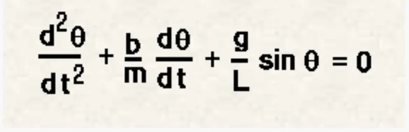
In the above equation,

• g = gravity in m/s²
• L = length of the pendulum in m
• m = mass of the ball in kg
• b = damping coefficient

Given Dimensions:

• L=1 metre
• M = 1 kg
• b=0.05
• g=9.81 m/s²

Theory:

A heavy body suspended by a light inextensible thread is called simple pendulum. This is impracticable, so in practice a small metal sphere is suspended from a rigid support using a cotton or silk thread. The point from which the bob is suspended is called point of suspension. The centre of gravity of the bob is called centre of oscillations. The distance between point of suspension and the centre of oscillations is called length of the pendulum.

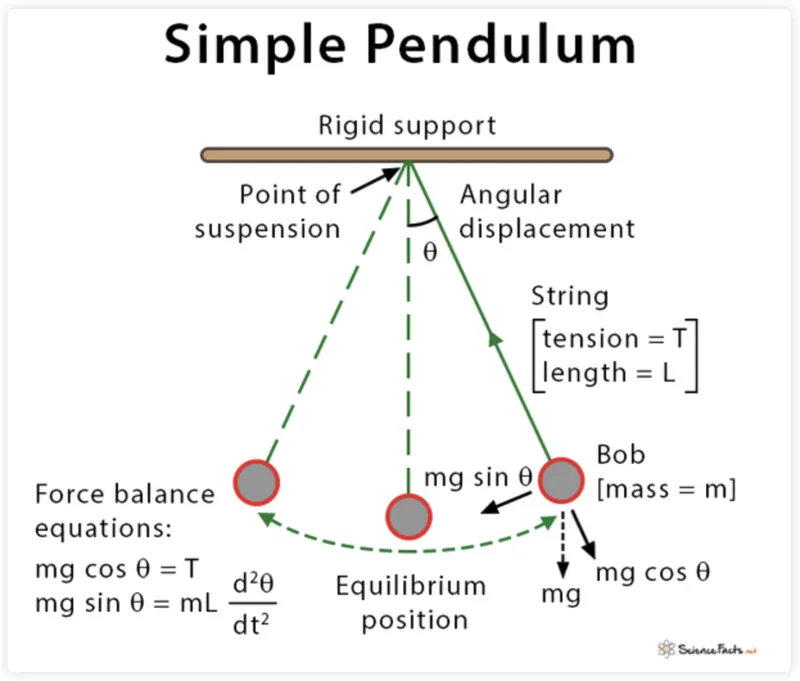
The weight of the bob acts vertically downwards and the tension in the string acts vertically upwards. These two forces are equal and opposite and the bob has equilibrium position in between. The bob displaced by an angle `theta` from equilibrium position.

Code for ode45 function call used in main program:

function [dtheta_dt] = ode_func(t,theta,b,g,l,m)

theta1=theta(1);
theta2=theta(2);

dtheta1_dt = theta2;
dtheta2_dt = -(b/m).* theta2 - (g/l).*sin( theta1);

dtheta_dt = [dtheta1_dt;dtheta2_dt];
end

MAIN PROGRAM:

% program to simulate motion of a simple pendulum

clear all
close all
clc

% inputs
b=0.05; % damping coefficient
g=9.81; % gravity in (m/s^2)
l=1; % length of the pendulum in metre
m=1; % mass of the ball in kg
ct=1;

% initial condition [initial position and initial velocity]
theta_0 = [0;3];

% time 
t_span = linspace(0,20,500);

% solving ODE
[t, results] = ode45(@(t,theta)ode_func(t,theta,b,g,l,m),t_span,theta_0);

% plots
figure(1)
plot(t,results(:,1))
hold on
plot(t,results(:,2))
xlabel('time')
ylabel('angular velocity and angular displacement')
legend('displacement', 'Angular velocity')
grid on
hold off

disp = results(:,1);
vel = results(:,2);

% pendulum motion animation

for i=1:length(t_span)
    figure(2)

%coordinates
x0=0;
y0=0; 
x1=-l*sind(results(i,1));
y1=-l*cosd(results(i,1));

plot ([x0 x1], [y0 y1],[-0.5 0.5], [0 0],'linewidth',2);
hold on
plot(x1,y1,'marker','o','markersize',25,'markerfacecolor','r','markeredgecolor','k')

% axis setting 
axis(gca,'equal')
grid on
pause(0.001)
hold off

M(ct)= getframe(gcf);
ct=ct+1;

end

% to create the videofile
movie(M)
videofile = VideoWriter('simple_pendulum.avi','uncompressed AVI');

% to open the videofile
open(videofile)

% to write the video file
writeVideo(videofile,M)

% to close the videofile
close(videofile)

CODE EXPLANATION:

• Set physics parameters of the pendulum like mass, length, gravity and damping coefficient.
• Set the initial conditions and timespan for which you want to run the simulation.
• To use the ode solver, use ode45 function with main inputs as (t and theta) while you use ode_func (the one we created earlier) with inputs as (t.theta,l,b,g.m) and t_span and theta_o as the initial conditions.
• These results are stored in an array of [t,results].
• Since results contain 2 components, angle displacement and velocity, to plot both the graphs, use the (:,1) and (:,2) property of MATLAB and plot those graphs.
• To create animation, Use a for loop so that we can get X and Y co-ordinates using trigonometry. Here, x0 and yo are the hinge points. Since they are (1.1) we have subtracted the co-ordinates of the bob from them so that proper rod of the pendulum can be seen.
• Use the pause () function to give a pause for every looping of values.
• Use movie making commands as per code to create a animation video.

ERRORS FACED:

1. 
2. 
3. 

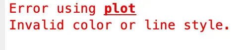
REASON TO FACE ERRORS:

1. The first error is faced because improper paranthesis is used inbetween the functions.
2. The second error is faced beecause invalid colour command is used while plotting.
3. The third error is faced because invalid value is used to define a sphere, '0' instead of 'o'.

SOLUTION TO RECTIFY OBTAINED ERRORS:

1. The first error can be rectified by using proper paranthesis in between the functions.
2. The second error can be rectified by using correct colour command recognised by MATLAB.
3. The third error can be rectified by using valid values to define a structure.

OUTPUT:

After rectifying the errors the obtained output is

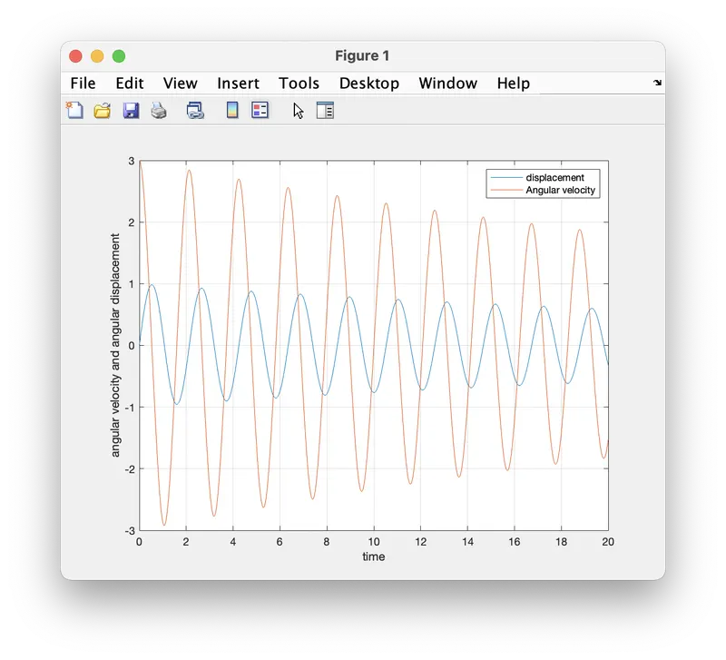
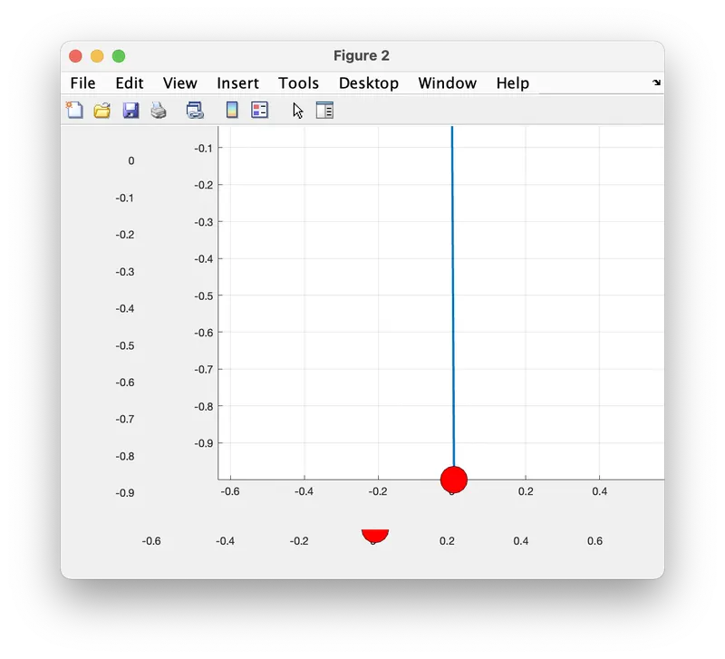
NOTE: The output in Figure 2 ia an screenshot image of the obtained animation. The Google Drive link for animated output is given below.

GOOGLE DRIVE LINK:

https://drive.google.com/file/d/1YDb0UFo8Rfp6H6nrbqAUydv1dk7BcfEt/view?usp=sharing

CONCLUSION:

• The reduction in velocity and Angle displacement is due to damping coefficient introduced in the Second order ODE of a simple pendulum.
• We have successfully solved the second order ODE.