Project 2 - Rankine cycle Simulator

RANKINE CYCLE SIMULATOR

Aim:

To write a MATLAB program to create the Rankine cycle simulator and obtain the required objectives.

Objective:

The objectives of writing the MATLAB program is shown below,

1. Create a Rankine cycle simulator by writing the MATLAB
2. Determine the state points and parameter using the available input parameters
3. Plot temperature and entropy or T-S diagram for the given set of inputs
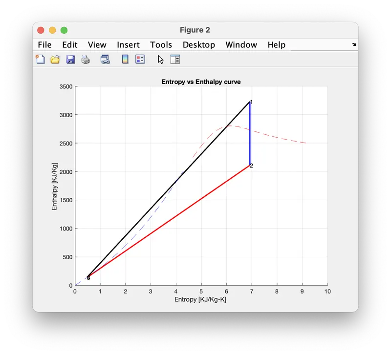
4. Plot enthalpy and entropy or H-S diagram for the given set of inputs

Introduction:

Rankine cycle- In simple words, a Rankine cycle is a kind of thermodynamic cycle that is normally used to determine or obtain the performance of some mechanical system like a steam turbine, reciprocating steam engines, etc. This is an ideal thermodynamic cycle. The various thermodynamic processes involved in the Rankine cycle is shown below,

1. Isentropic expansion thermodynamic process
2. lsobaric heat rejection thermodynamic process
3. Isentropic compression thermodynamic process
4. Isobaric heat transfers thermodynamic process

Steam turbine- In simple word, a mechanical device is known as steam turbine, if it obtains thermal or heat energy from steam (that is in the pressurized form) and utilize it to do some mechanical work and provide it in a rotating shaft. The various types of a steam turbine are shown below,

1. Back-pressure steam turbine
2. Extraction steam turbine
3. Condensing steam turbine

Required Diagram:(Basic schematic of a Rankine cycle)

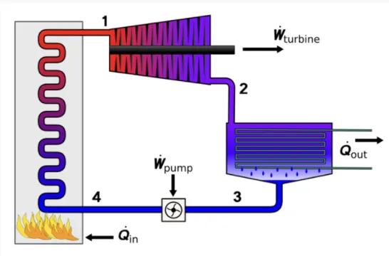
Condenser- In simple words, a mechanical device is known as a condenser, if it condenses a gaseous chemical element (like steam) into its liquid form with the help of cooling. The various types of the condenser are shown below,

1. Water-cooled condenser
2. Air-cooled condenser
3. Evaporative condenser

Pump- A mechanical device is known as the pump if it is used to moves liquid, gasses, or slurries from one place to another place or lower heat to the upper head or vice versa. The various types of pump are shown below,

1. Centrifugal pump
2. Reciprocating pump
3. Rotary pump
4. Screw pump

Boiler- A mechanical device is known as a boiler if it is used to generate steam by heating water with the help of provided thermal energy. The various types of boiler are shown below,

1. Water-tube boiler
2. Fire-tube boiler

Turbine- A mechanical device is known as a turbine, if it is used to generate mechanical work or mechanical energy from moving fluid-like, water, steam, air, etc. The various types of turbines are shown below,

1. Steam turbine
2. Kaplan turbine
3. Francis turbine

Process Diagram of Rankine Cycle is shown below:

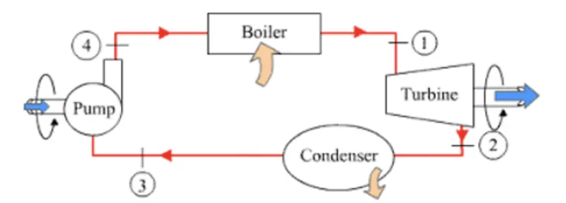
1. Process (1-2) Isentropic expansion thermodynamic process- The vapor is expanded in the turbine, thus producing work that may be converted to electricity. In practice, the expansion is limited by the temperature of the cooling medium and by the erosion of the turbine blades by liquid entrainment in the vapor stream as the process moves further into the two-phase region. Exit vapor qualities should be greater than 90% to increase the life of the turbine blade.

2. Process (2-3) Isobaric heat rejection thermodynamic process- The vapor-liquid mixture leaving the turbine (2) is condensed at low pressure, usually in a surface condenser using cooling water. In well designed and maintained condensers, the pressure of the vapor is well below atmospheric pressure, approaching the saturation pressure of the operating fluid at the cooling water temperature.

3. Process (3-4) Isentropic compression thermodynamic process- The pressure of the condensate is raised in the feed pump. Because of the low specific volume of liquids, the pump work is relatively small and often neglected in thermodynamic calculations.

4. Process (4-1) Isobaric heat transfer thermodynamic process- High-pressure liquid enters the boiler from the feed pump (4) and is heated to the saturation temperature. Further addition of energy causes evaporation of the liquid until it is fully converted to saturated steam (1).

Here the given input values are,

• Turbine Inlet temperature = 400° C
• Turbine Inlet Pressure = 30 bar
• Turbine Outlet Pressure = 0.05 bars = Condenser Inlet Pressure

MAIN CODE:

clear all
close all
clc

% taking inputs
P1 = input('Enter the Pressure at the Turbine Inlet (in bar): ');
T1 = input('Enter the Temperature at the Turbine Inlet (in Degree Celsius): ');
P2 = input('Enter the Pressure at the Condenser (in bar): ');

% conditions at the turbine inlet
T1_sat = XSteam('Tsat_p',P1);
if T1 > T1_sat
h1 = XSteam('h_pt',P1,T1);
s1 = XSteam('s_pt',P1,T1);
elseif T1 == T1_sat
h1 = XSteam('hV_p',P1);
s1 = XSteam('sV_p',P1);
else
disp('enter higher value of temperature')
end

% conditions at turbine outlet
s2 = s1;
s2_sat = XSteam('sV_p',P2);
if s2 < s2_sat
s2_f = XSteam('sL_p',P2);
s2_g = XSteam('sV_p',P2);

% s2 = s_f + x(s_g - s_f)
% x = vapour fraction
x2 = (s2 - s2_f)/(s2_g - s2_f);
h2_f = XSteam('hL_p',P2);
h2_g = XSteam('hV_p',P2);
h2 = h2_f + x2*(h2_g - h2_f);
T2 = XSteam('Tsat_p',P2);
else
x2 = 1;
h2 = XSteam('hV_p',P2);
T2 = XSteam('Tsat_p',P2);
end

% conditions at condensor outlet/ pump inlet
P3 = P2;
T3 = XSteam('Tsat_p',P3);
h3 = XSteam('hL_p',P3);
s3 = XSteam('sL_p',P3);
v3 = XSteam('vL_p',P3);

% conditions at pump outlet
s4 = s3;
P4 = P1;
v4 = XSteam('v_ps',P4,s4);
Cp = XSteam('Cp_ps',P4,s4);
Cv = XSteam('Cv_ps',P4,s4);
g = Cp/Cv;    % gamma
T4 = T3*((P3/P4)^((1-g)/g));
W_p = v3*(P4 - P3)*100;  % work done by pump
h4 = h3 + W_p;

% considering point 5 and 6 to complete the curve
T5 = XSteam('Tsat_p',P4);
s5 = XSteam('sL_p',P4);
T6 = T5;
s6 = XSteam('sV_T',T6);

% Work done, heat and efficiency
% assuming mass flow rate = 1
W_t = h1 - h2;       % work done by turbine
W_net = W_t - W_p;   % net work done
Q_in = h1 - h4;      % heat added
Q_out = h2 - h3;     % heat rejected
eta = W_net/Q_in;    % efficiency
SSC = 3600/W_net;    % specific steam consumption (SSC)
BWR = W_p/W_t;

% plotting
t = linspace(0,600,1000);
% for plotting saturation curves
for i = 1:length(t)
s_l(i) = XSteam('sL_T',t(i));
s_v(i) = XSteam('sV_T',t(i));
h_l(i) = XSteam('hL_T',t(i));
h_v(i) = XSteam('hV_T',t(i));
end
% plotting T-S curve
figure(1)
hold on
plot(s_l,t,'--','color','b')
plot(s_v,t,'--','color','r')
plot([s1,s2],[T1,T2],'linewidth',2,'color','b')
plot([s2,s3],[T2,T3],'linewidth',2,'color','r')
plot([s3,s4],[T3,T4],'linewidth',2,'color','y')
plot([s4,s5],[T4,T5],'linewidth',2,'color','k')
plot([s5,s6],[T5,T6],'linewidth',2,'color','k')
plot([s6,s1],[T6,T1],'linewidth',2,'color','k')
text(s1,T1,'1')
text(s2,T2,'2')
text(s3,T3,'3')
text(s4,T4,'4')
text(s5,T5,'5')
text(s6,T6,'6')
xlabel('Entropy [KJ/Kg-K] ')
ylabel('Temperature [C]')
title('Entropy vs Temperature curve')
grid on
hold off

% plotting h-s curve
figure(2)
hold on
plot([s1,s2],[h1,h2],'linewidth',2,'color','b')
plot([s2,s3],[h2,h3],'linewidth',2,'color','r')
plot([s3,s4],[h3,h4],'linewidth',2,'color','y')
plot([s4,s1],[h4,h1],'linewidth',2,'color','k')
plot(s_l,h_l,'--', 'color','b')
plot(s_v,h_v,'--','color','r')
text(s1,h1,'1')
text(s2,h2,'2')
text(s3,h3,'3')
text(s4,h4,'4')
xlabel('Entropy [KJ/Kg-K] ')
ylabel('Enthalpy [KJ/Kg] ')
title('Entropy vs Enthalpy curve')
grid on
hold off

% getting the output screen
disp('RESULTS: ')
disp('At state point 1: ')
fprintf('P1 = %.2f bar \n',P1)
fprintf(['T1 = %.2f' char(176) 'C \n'],T1)
fprintf('h1 = %.2f kJ/kg \n',h1)
fprintf('s1 = %.2f kJ/kgKN \n',s1)
disp(' ')
disp('At state point 2: ')
fprintf('P2 = %.2f bar \n',P2)
fprintf(['T2 = %.2f' char(176) 'C \n'],T2)
fprintf('h2 = %.2f kJ/kg \n',h2)
fprintf('s2 = %.2f kJ/kgKN \n',s2)
disp(' ')
disp('At state point 3: ')
fprintf('P3 = %.2f bar \n',P3)
fprintf(['T3 = %.2f' char(176) 'C \n'],T3)
fprintf('h3 = %.2f kJ/kg \n',h3)
fprintf('s3 = %.2f kJ/kgKN \n',s3)
disp(' ')
disp('At state point 4: ')
fprintf('P4 = %.2f bar \n',P4)
fprintf(['T4 = %.2f' char(176) 'C \n'],T4)
fprintf('h4 = %.2f kJ/kg \n',h4)
fprintf('s4 = %.2f kJ/kgKN \n',s4)
disp(' ')

fprintf('Work done by turbine = %.2f kJ/kg \n', W_t)
fprintf('Work done by pump = %.2f kJ/kg \n', W_p)
fprintf('Net work output = %.2f kJ/kg \n', W_net)
fprintf('Thermal efficiency = %.2f \n', eta)
fprintf('Back-work ratio = %f \n', BWR)
fprintf('Specific Steam Conductivity = %.2f kg/kWh \n', SSC)

CODE EXPLANATION:

• The values of "P1", "T1" and "P2" were given as input. And the temperature value array “t" was created using "linspace" command.
• The using the provided "XSteam" library the values of various physical parameters i.e. Enthalpy ,Entropy , Saturated liquid/vapour - enthalpy/entropy ,stauration temperature at 4 state points were calculated.
• Then using basic relations between work and physical parameters and "basic mathematical operations in octave" the "W_net", "back_wr'" etc. were calculated.
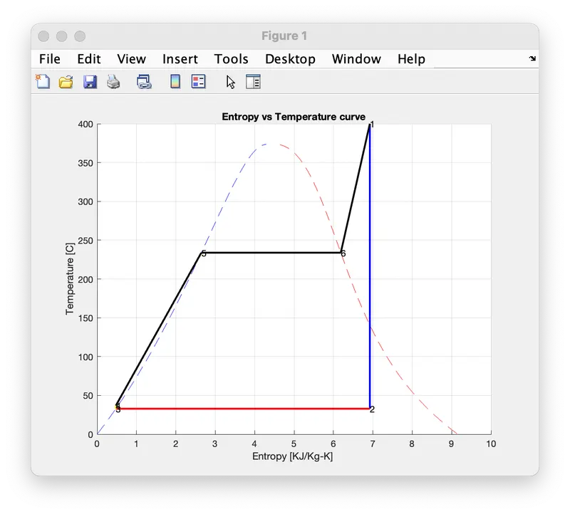
• Next step was to plot the T-s curve . Here again we used the provided "XSteam” library function to plot the T-s Curve at different temperature array values. Then along with the state points the curve was plotted.
• Similarly, the T-s curve was plotted. Here again we used the provided "XSteam" library function to plot the h-s Curve at different temperature array values. Then along with the state points the curve was plotted.
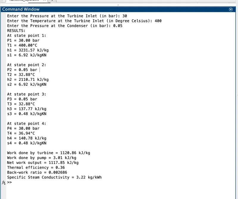
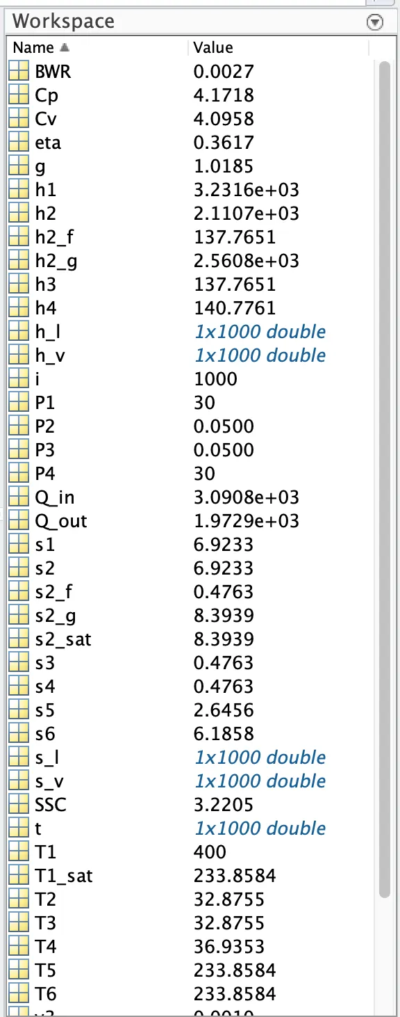
• The values of physical parameters at the state points were displayed in the output window. This was done for all the "4" defining state points in similar way.
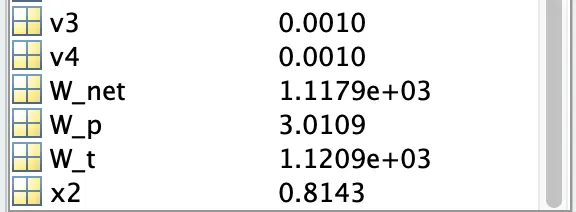
• Then the final results i.e. "W_net","W_turbine","W-pump",“back_wr","ssc","therm _eff" were printed.

OUTPUT:

• COMMAND WINDOW:

• T-S CURVE:

• h-S CURVE:

• WORKSPACE:

ERRORS:

• No major errors were faced during the project, only typos and wrong uses of brackets which is rectified immediately.

REFERENCES:

• NPTEL
• BASIC RANKINE CYCLE