Week 3 - Solving second order ODEs

AIM;

To solve the second order ODE function using matlab which depicts the motion of the pendulum and to create an animation of the same.

Objective;

To write a program that solves the following ODE. this ODE represents the equation of motion of a simple pendulum with damping

Formula;

(d^2/dt^2)+b/m(dtheta/dt)+g/l sin(theta) = 0

in the above equation,

g = gravity in (m/s^2)

l = length of the pendulum in m

m = mass of the ball in kg

b = damping coefficient

Fixed parameter;

b = 0.05

g = 9.81

l = 1

m = 0.1

time period = 0-20sec

angular displacement = 0

angular velocity = 3rad/sec

time t = 0

FUNCTION CODE;

function [dtheta_dt] = ode_funs(~,theta,b,g,l,m)
  
      theta1 = theta(1);
      theta2 = theta(2);
      dtheta1_dt = theta2;
      dtheta2_dt = -(b/m)*theta2 - (g/l)*sin(theta1);
      dtheta_dt = [dtheta1_dt; dtheta2_dt];
end

EXPLANATION;

• In this function program, the second order ode is simplified to the first order ode by introducing the term theta1 & theta2.
• Then the theta1 & theta2 is differentiated and the dtheta_dt gives a column matrix.

MAIN PROGRAMM;

close all
clc



b=0.05;
g=9.81;
l=1;
m=0.1;

%initial condition

theta_0=[0;5];

%time points

t_span=linspace(0, 10, 500);

%solve ODE

[t, results] = ode45(@(t,theta) ode_funs(t,theta,b,g,l,m),t_span,theta_0);

%plotting

plot(t, results(:,1))
hold on
plot(t, results(:,2))

%Animation
ct = 1;
for i = 1:length(results(:,1))
    x0 = 0;
    y0 = 0;
    x1 = l*sind(results(i,1)+pi);
    y1 = l*cosd(results(i,1)+pi);

    plot([x0 x1],[y0 y1],'-o','MarkerSize',10,'MarkerFaceColor','r','MarkerEdgeColor','r','linewidth',4)
    axis([-2 2 -2 2])
    hold on
    plot([-1 1],[0 0],'linewidth',5,'color','[0 0.3 0]')
    M(ct) = getframe(gcf);
    hold off
    ct = ct + 1;
end

%movie & videofile

movie(M)
v_f = VideoWriter('Pendulum_Challenge.avi','Uncompressed AVI');
open(v_f)
writeVideo(v_f, M)
close(v-f)

EXPLANATION;

• In the above programm the fixed parameters are length, mass, damping coefficient and accelerating due to gravity.
• Time and angle are given as the initial condition.
• In the tspan command, 200 values aare taken in between 0 to 20 time period.
• Using the ode 45 command ode function is introduced.
• Using the plot command velocity and displacement is plotted in the y axis against time in the x axis.
• Using the for loop command the mass at various pooints and various times are marked in the graph and are plotted.
• Using the movie command the plot is saved as an uncompressed avi file.

ERROR;

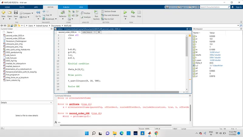
Myself i faced alot of error which are occured due to my carelessness i keep on typing the code not even look into the screen which show off error while run the program, after that i go through step by step and found all those minor error which cause major impact in running the programm

SCREENSHOT;

RESULT;

Hence, the second order ode function using matlab which depicts the motion of the pendulum and the anmination of the same are done.