Project 2 - Rankine cycle Simulator

AIM:

To Create a Rankine Cycle Simulator using MATLAB.

OBJECTIVE:

• Calculate each state points of the Rankine Cycle (any type of your choice) based on user inputs.

• Plot the corresponding T-s and h-s plots for the given set of inputs.

• Calculate Efficiency.

THEORY:

The Rankine cycle is an idealized thermodynamic cycle of a heat engine that converts heat into mechanical work while undergoing a phase change. It is an idealized cycle in which friction losses in each of the four components are neglected. The heat is supplied externally to a closed loop, which usually uses water as the working fluid.

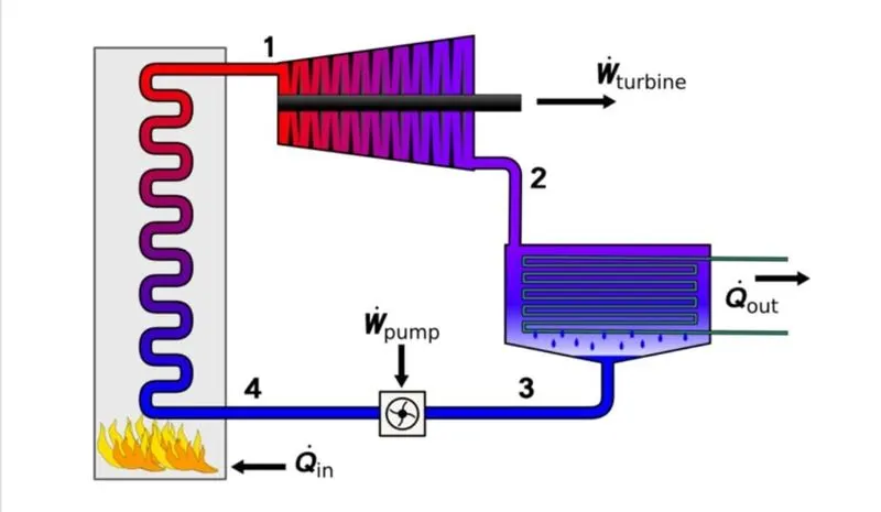
Four components of the Rankine cycle:

1. Turbine

2. Condenser

3. Pump

4. Boiler

Four processes of the Rankine cycle:

1-2: Isentropic Expansion

Turbine (1-2): Superheated steam enters into the Turbine and expands isentropically resulting in the production of work. The shaft of the turbine is connected to the generator. This results in the production of electricity i.e Mechanical energy gets converted into electric energy. Work produced by the turbine, Wt = m(h1-h2)K

2-3: Constant Pressure Heat Rejection

Condenser (2-3): The expanded vapour is then passed through a condenser, where it gets condensed and converts into liquid again. This liquid is again pumped to the boiler.

Qr = m(h2-h3)K

3-4: Isentropic Compression by the Pump

Pump (3-4): The water enters into the pump in a saturated state. Then the liquid is compressed isentropically until it meets the boiler pressure. Work done by the pump is, Wp = m(h3 - h4)K

4-1: Constant Pressure Heat Addition

Boiler (4-1): The water enters into the boiler as compressed and leaves as superheated from the boiler. Thus the phase changes from liquid to vapour. The heat supplied by the boiler is

Qb=m(h1-h4)K

Here we take mass flow rate m = 1 for this code.

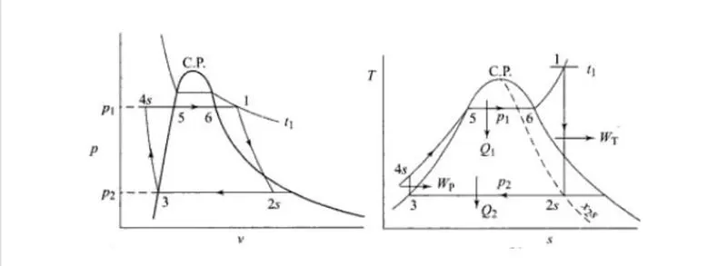
• The efficiency of the Steam Cycle is given

by

`ef`= Wn/Q1=Wt-Wp/Q1

Applying the Steady Flow Energy Equation (SFEE) to all the process, neglecting the Friction losses and changs in Kinetic & Potential Energy,

• Q1=hl-h4 @Boiler
• Wt=hl-h2 @Turbine
• Q2=h2-h3 @Condenser
• Wp-h4-h3 @Pump
• • The Capacity of the Steam Plant is often expressed interms of Steam Rate (SR) or Specific Steam Consumption (SSC)

S. S. C. = (3600/Wn)(kg/kWh)

Required inputs;

• Turbine inlet temperature = 400 c
• Turbine inlet pressure = 30 bars
• Turbine outlet pressure = 0.05bars = Condenser inlet pressure

MATLAB CODE:

close all 
clc

%print process descripton
fprintf('1-2isobaric heat transfer/n')
fprintf('2-3isentropic expansion/n')
fprintf('3-4isobaric heat rejection/n')
fprintf('4-1isentropic compression/n')

%step 1:Enter inputs
p1 = input('30bars:');
T1 = input('400c:');
p2 = input('0.05bars:');

%step 2: calculate each state point values
%state point 1
h1 = Xsteam('h_pt',p1,T1);
s1 = Xsteam('s_pt',p1,T1);

%step 3:state point 2
s2 = s1;

sf2 = Xsteam('sL_p',p2);
sg2 = Xsteam('sV_p',p2);
hf2 = XSteam('hL_p',p2);
hg2 = Xsteam('hV_p',p2);
s2 = sg2;
h2 = hg2;
T2 = Xsteam('T_hs',h2,s2);

%step 4: state point 3
T3 = T4;
p3 = p2;
s3 = Xsteam('sL_T',T3);
h3 = Xsteam('hL_T',T3);
v3 = Xsteam('vL_p',p2);

%step 5: state point 4
p4 = p1;
s4 = s3;
Cp4 = Xsteam('Cp_ps',p4,s4);
Cv4 = Xsteam('Cv_ps',p4,s4);
gamma = Cp4/Cv4;
r = (gamma - 1)/gamma;
T4 = T3*(p4/p3)^r;

%step 6: calculate other output values.
Wt = h1- h2;
Wp = v3*(p1-p2)*100;
h4 = Wp + h3;
W_net = Wt-Wp;
Qs = h1 - h4;
N_per = (W_net/Qs)*100;
steam_rate = 3600/(Wt - Wp);

%step 7: state point 5 and 8 which help in plotting
T5 = Xsteam('sL_p',p1);
T6 = T5;
s5 = Xsteam('sL_p',p1);
s6 = Xsteam('sV_p',p1);
h5 = Xsteam('hL_p',p1);
h6 = Xsteam('hV_p',p1);

%step 8: print all state point values to show.
fprintf('\n------result----/n')
fprintf( 'at state point 1 : \nP1 is : %4.2f bar\nT1 is : %4.2f degree celcius\nH1 is : 4.2f kj/kg\nS1 is : %4.2f kj/kgk\n\n' ,p1,T1,h1,s1)
fprintf( 'at state point 2 : \nP2 is : %4.2f bar\nT2 is : %4.2f degree celcius\nH2 is : 4.2f kj/kg\nS2 is : %4.2f kj/kgk\n\n' ,p2,T2,h2,s2)
fprintf( 'at state point 3 : \nP1 is : %4.2f bar\nT3 is : %4.2f degree celcius\nH3 is : 4.2f kj/kg\nS3 is : %4.2f kj/kgk\n\n' ,p3,T3,h3,s3)
fprintf( 'at state point 4 : \nP1 is : %4.2f bar\nT4 is : %4.2f degree celcius\nH4 is : 4.2f kj/kg\nS4 is : %4.2f kj/kgk\n\n' ,p4,T4,h4,s4)
fprintf('Wt is :%4.2f kj/kg\nWp is : %4.2f kj/kg\nWnet is : %4.2f kj/kg\nNtherm is : %4.2f percent\nS.S.C is : %4.2f kg/kWh' ,Wt,Wp,W_net,N_per,steam_rate)

%step 9:plot T-S diagram
subplot(1,2,1)
T_rankie = linspace(T5,T1,5000);
for i = 1 : length(T_rankie)
    s_rankie(i) = Xsteam('s_pT',p1,T_rankie(i));
end
plot([s1 s2 s3 s4 s5 s6 s_rankie],[T1 T2 T3 T4 T5 T6 T_rankie],'linewidth',1.5);
hold on
T_curve + linspace(1,400,500);
for i = 1 : length(T_curve)
    s_l(i) = Xsteam('sL_T',T_curve(i));
    s_v(i) = Xsteam('sV_T',T_curve(i));
    h_l(i) = xsteam('hL_T',T_curve(i));
    h_v(i) = Xsteam('hV_T',T_curve(i));
end

plot(s_l,T_curve);
plot(s_v,T_curve);
text(s1,T1,'1','FontSize',15)
text(s2,T2,'2','FontSize',15)
text(s3,T3,'3','FontSize',15,'HorizontalAlignment','right','VerticalAlignment','top')
text(s4,T4,'4','FontSize',15,'HorizontalAlignment','right','VerticalAlignment','bottom')
text(s5,T5,'5','FontSize',15)
text(s6,T6,'6','FontSize',15)
xlabel('entropy in kj/kgk');
ylabel('temperature in degree celcius');

%step 10:plot H-s diagram
subplot(1, 2, 2)
plot([s1 s2 s3 s4 s1],[h1 h2 h3 h4 h1],'LineWidth',2)
hold on
plot(s_v,h_v,'Color','r')
plot(s_l,h_l,'Color','r')
text(s1,h1,'1','FontSize',15)
text(s2,h2,'2','FontSize',15)
text(s3,T3,'3','FontSize',15,'HorizontalAlignment','right','VerticalAlignment','top')
text(s4,T4,'4','FontSize',15,'HorizontalAlignment','right','VerticalAlignment','bottom')
xlabel('entropy in kj/kgk')
ylabel('enthalpy in kj/kg')

COMMAND WINDOWS:

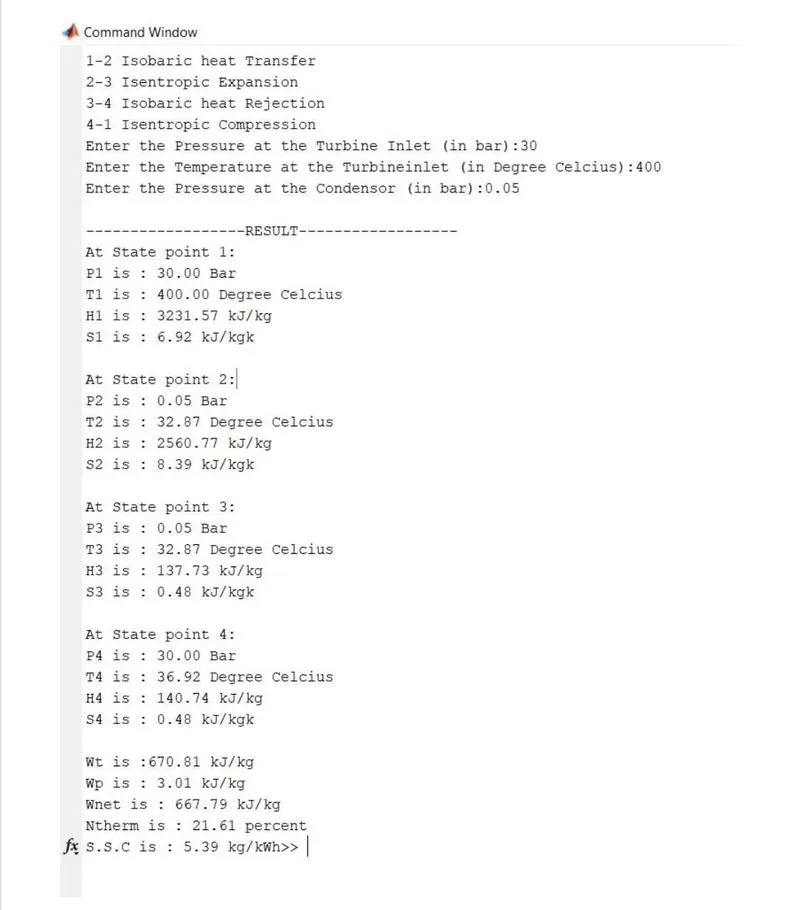
RESULTANT PLOT:

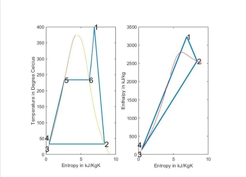
RESULT:

The rankie cycle plots have generated by calculating the state points,efficiency and the output is printed in the command window.